Permeability Imaging via DSS Strain Inversion (Research Log)
- Permeability Imaging via DSS Strain Inversion
- 2026-01-14
- Bug fixed
- 2026-01-16
- 2026-01-17
- 2026-01-19
- Optimization result
- Retake perm imaging
- The Jacobian
- Forward file
- 2026-03-09
- 2026-03-11
- 2026-03-13
- 2026-03-14 - prompt
- 2026-03-16
- 2026-03-17
- The mystery of optimizer
- 2026-04-02
- 2026-04-03
- 2026-04-04
- 2026-04-07
- 2026-04-08
- 2026-04-16
- 2026-04-17
- 2026-04-21
- 2026-05-04
- 2026-06-01
- 2026-06-03
- 2026-06-08
- 2026-06-12
Permeability Imaging via DSS Strain Inversion
This is a lightly-edited research log (Jan–Jun 2026) documenting my work on imaging reservoir permeability by inverting distributed strain sensing (DSS) data from a fiber-optic interference test. The workflow couples a MOOSE forward poro-mechanical model with an adjoint-based gradient and a Python (L-BFGS-B) outer optimizer, built on top of my fibeRIS toolkit. Entries are dated; figures and console output are kept as captured during the work.
2026-01-14
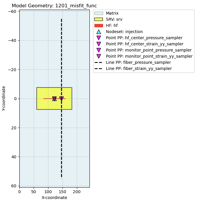
Let’s fix the final bug. Why the diffusion pattern is not observable? Why the pressure curve is not functioning as we thought?
- I am comparing the
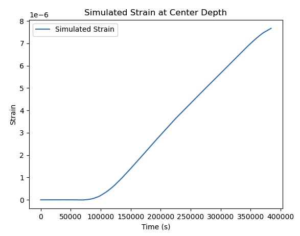
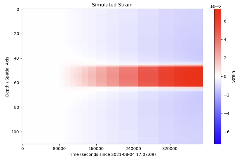
107_3xFrac_revised.pywith the model generator. Test 1: - srv porosity from 0.032 → 0.1
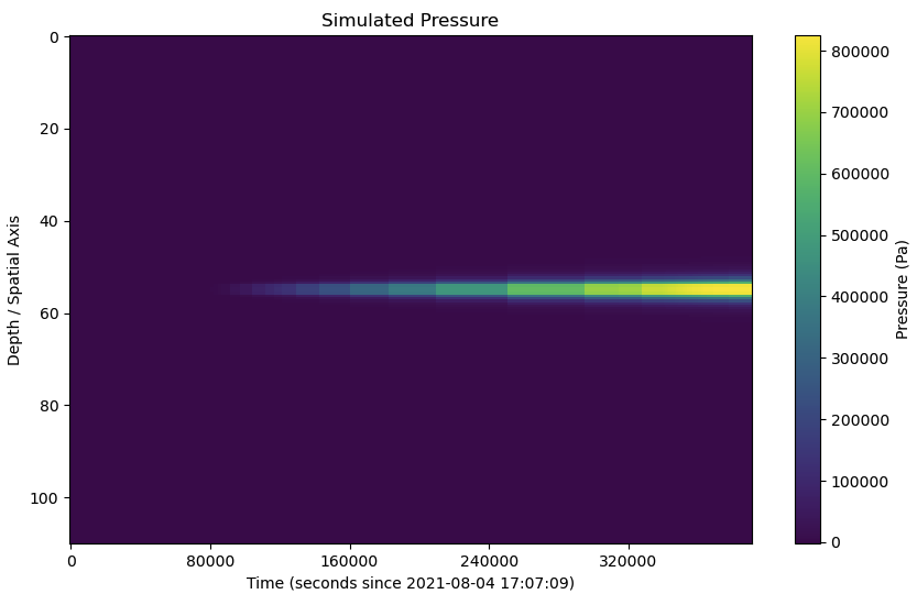
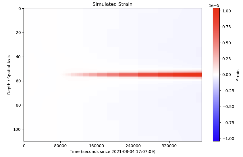
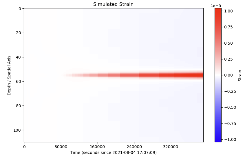 result from porosity = 0.032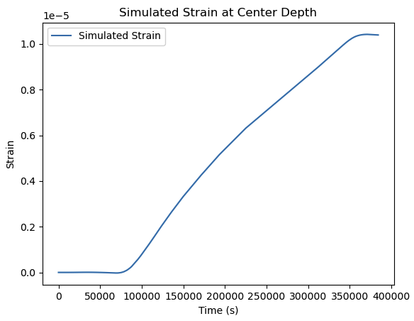
 Test 2:
 - SRV size from 5 ft to 50 ft
 TBH it’s not working as expected.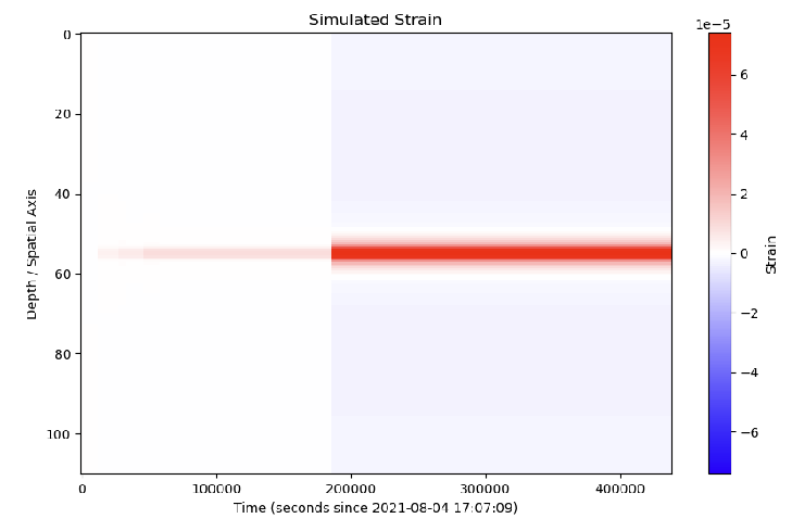
- Next step, test the pressure profile. Use a dedicated profile will work or not? I don’t think so TBH I kinda suspect there are other fatal bugs in v1.
Bug fixed
The full profile will return a correct result. This one is the strain with simulation during production
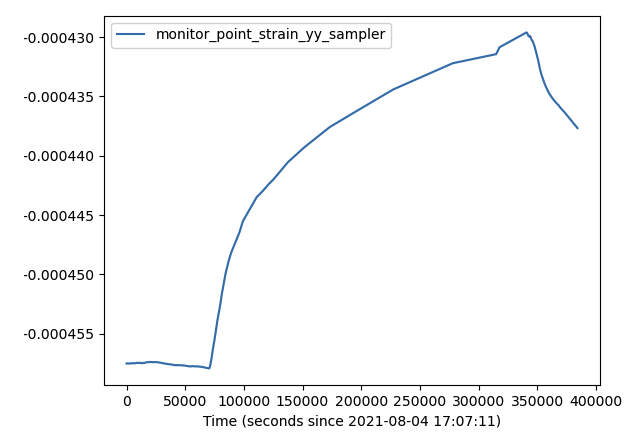 While this one is without simulating the production.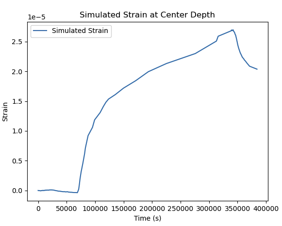
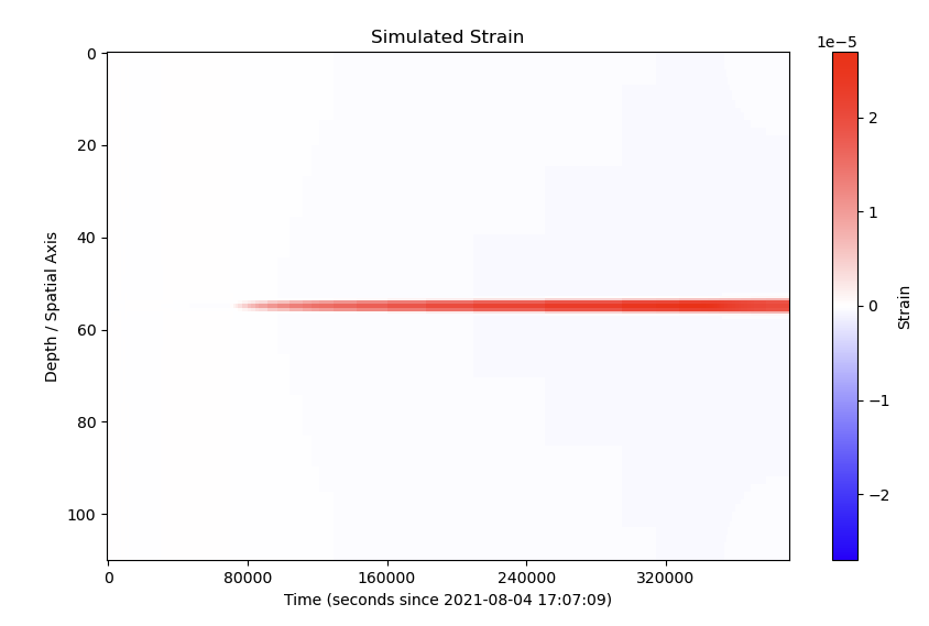
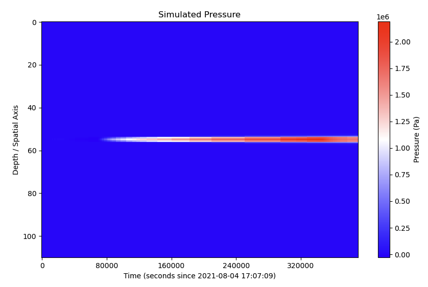
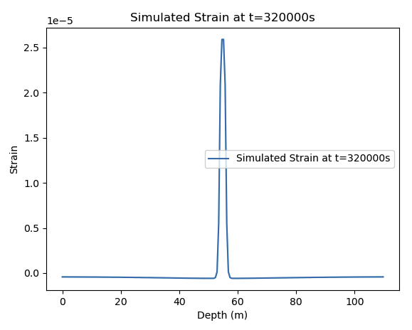 Zoom-in: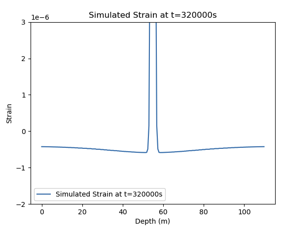
2026-01-16
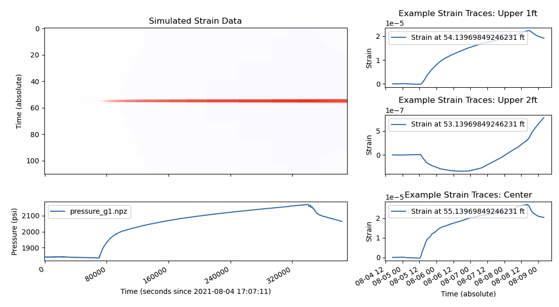
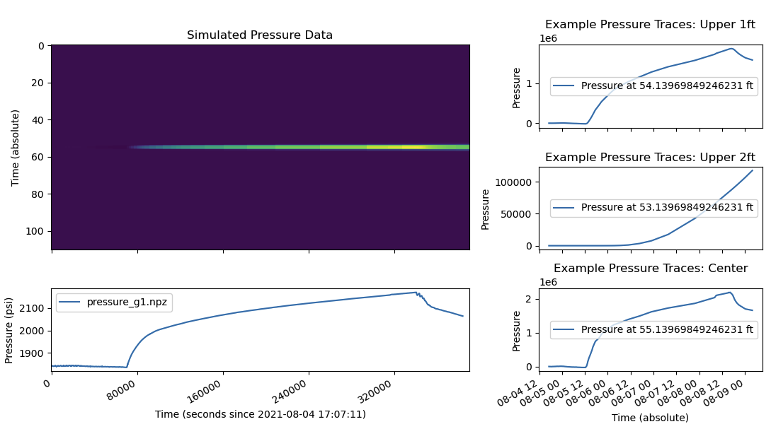
We can start to do the optimization. First a better visualization can help us a lot.
2026-01-17
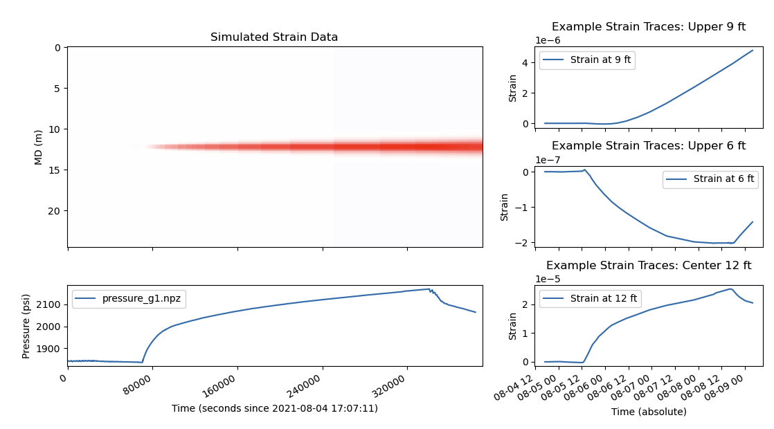
I started to think about how we can create the figure. I would like to say there will be
- Strain plot, the result within 30 ft, upper 1 ft chan, lower 1 ft chan, center chan, also a time slice
- Comparison of strain plot: the simulation and real data. waterfall plot, channel data comparison.
2026-01-19
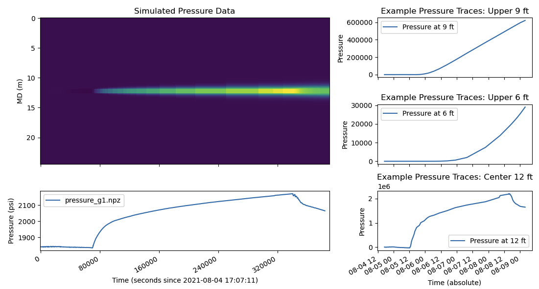
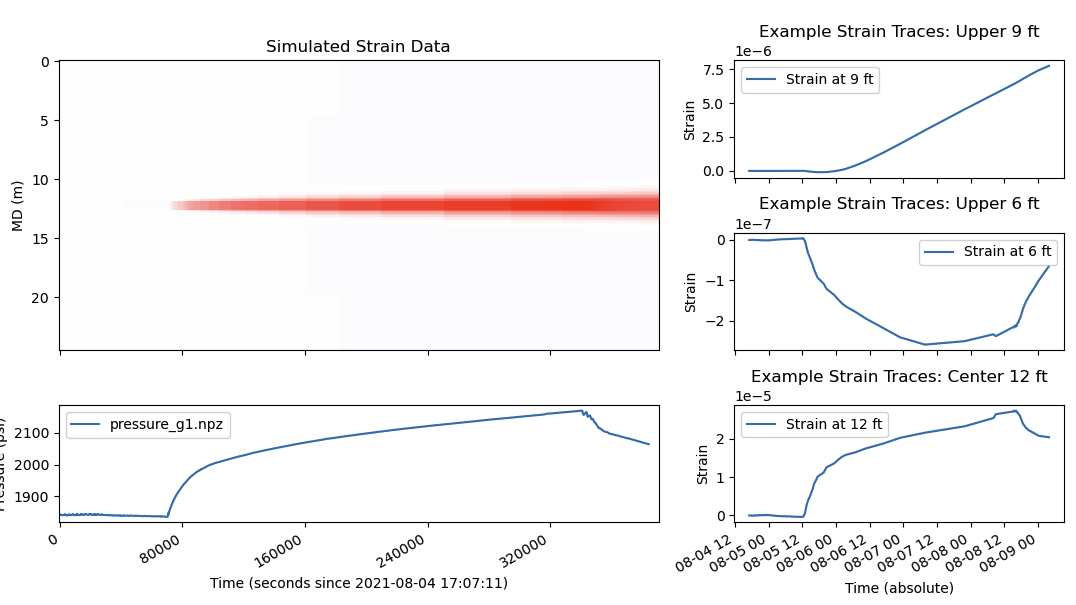
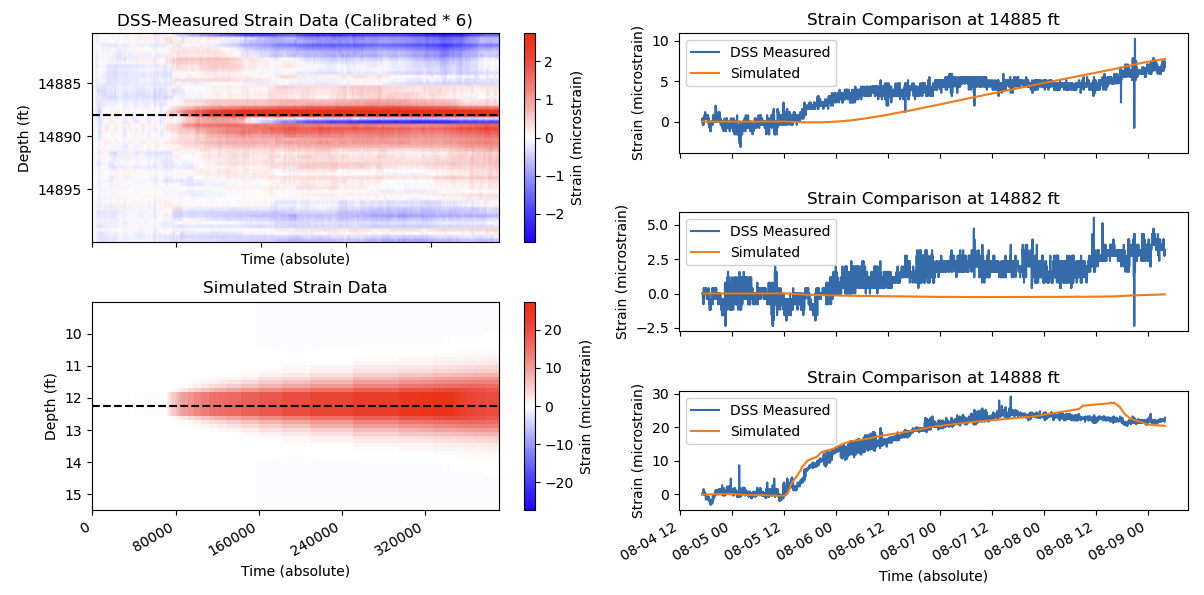
 I’m creating the figure showing the difference between rael data
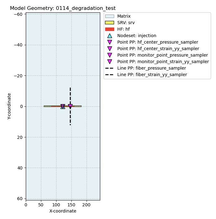
Initial model
I will optimize the parameter based on this initial model:
Optimization result
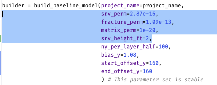
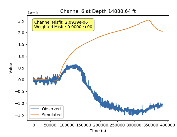
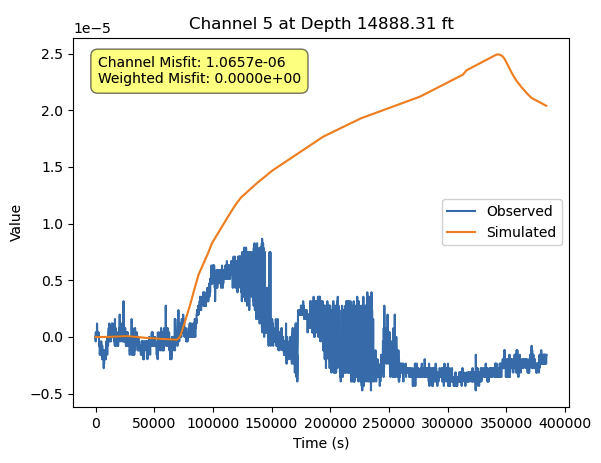
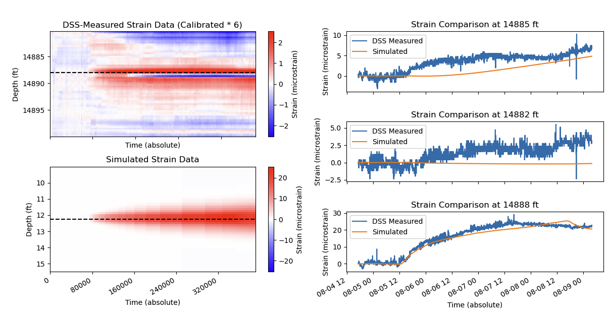
The best result is found in iteration 3. Which has ```python Iteration: 3 {‘srv_perm’: 2.386418878005603e-16, ‘fracture_perm’: 1.0025956902289557e-14, ‘srv_height_ft’: 1.1429006806487336} Total Misfit: 1.520372345579617e-06
2.6891e-08 3.6769e-08 3.7928e-08 1.4574e-07 1.6512e-08 0.0000e+00 0.0000e+00 6.7966e-07 2.2051e-07 1.0568e-07 1.5339e-07 5.6034e-08 2.0076e-08 1.2080e-08 9.1020e-09
## 2026-01-27
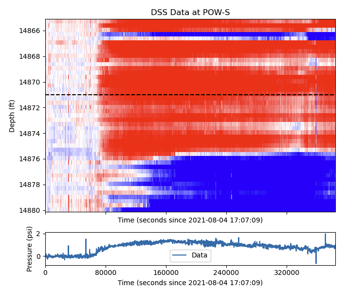
I’m migrating single optimization to multiple hydraulic fracture optimization. I’ve created every single tool we need for the task. So let’s first select several fractures within 100ft.
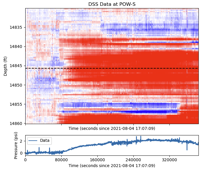
14845.67 \[1, 1, 1, 2, 1, 1, 1\] range=10
14871.00 \[1,1,1,2,1,1,1\] range = 10
## 2026-01-28
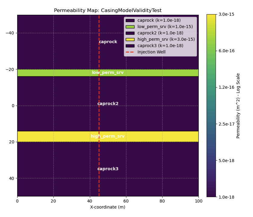
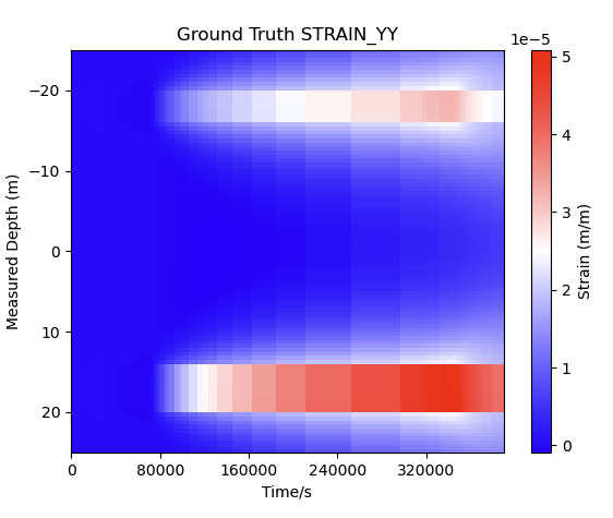
I suppose we need to update the whole model structure to image the permeability. It will be uniformly sampled, every stripe has it permeability.
## 2026-02-11
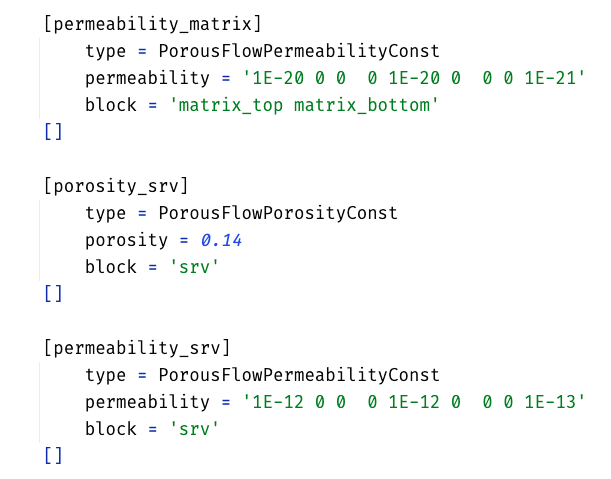
### GT model

## 2026-02-13
I’m working on generation of that “initial” optimizer. We now have the heat case, to perform the optimization.
The `main.i`
```toml
[Optimization]
[]
[Mesh]
type = GeneratedMesh
dim = 2
nx = 10
ny = 10
xmax = 2
ymax = 2
[]
[OptimizationReporter]
type = GeneralOptimization
objective_name = objective_value
parameter_names = 'p1'
num_values = '1'
initial_condition = '7'
lower_bounds = '0'
upper_bounds = '10'
[]
[Reporters]
[main]
type = OptimizationData
measurement_points = '0.2 0.2 0
0.8 0.6 0
0.2 1.4 0
0.8 1.8 0'
measurement_values = '226 254 214 146'
[]
[]
[Executioner]
type = Optimize
tao_solver = taoblmvm
petsc_options_iname = '-tao_gatol'
petsc_options_value = '0.0001'
verbose = true
[]
[MultiApps]
[forward]
type = FullSolveMultiApp
input_files = forward.i
execute_on = "FORWARD"
clone_parent_mesh = true
[]
[adjoint]
type = FullSolveMultiApp
input_files = adjoint.i
execute_on = "ADJOINT"
clone_parent_mesh = true
[]
[]
[Transfers]
[toForward]
type = MultiAppReporterTransfer
to_multi_app = forward
from_reporters = 'main/measurement_xcoord
main/measurement_ycoord
main/measurement_zcoord
main/measurement_time
main/measurement_values
OptimizationReporter/p1'
to_reporters = 'measure_data/measurement_xcoord
measure_data/measurement_ycoord
measure_data/measurement_zcoord
measure_data/measurement_time
measure_data/measurement_values
params/p1'
[]
[fromForward_mesh]
type = MultiAppCopyTransfer
from_multi_app = forward
to_multi_app = adjoint
source_variable = 'temperature'
variable = 'temperature_forward'
[]
[fromForward]
type = MultiAppReporterTransfer
from_multi_app = forward
from_reporters = 'measure_data/misfit_values measure_data/objective_value'
to_reporters = 'main/misfit_values OptimizationReporter/objective_value'
[]
[toAdjoint]
type = MultiAppReporterTransfer
to_multi_app = adjoint
from_reporters = 'main/measurement_xcoord
main/measurement_ycoord
main/measurement_zcoord
main/measurement_time
main/misfit_values
OptimizationReporter/p1'
to_reporters = 'misfit/measurement_xcoord
misfit/measurement_ycoord
misfit/measurement_zcoord
misfit/measurement_time
misfit/misfit_values
params/p1'
[]
[fromAdjoint]
type = MultiAppReporterTransfer
from_multi_app = adjoint
from_reporters = 'adjoint_grad/inner_product'
to_reporters = 'OptimizationReporter/grad_p1'
[]
[]
[Outputs]
csv = true
[]
The forward modeling:
[Mesh]
[]

[Variables]
  [temperature]
  []
[]

[Kernels]
  [heat_conduction]
    type = MatDiffusion
    variable = temperature
    diffusivity = thermal_conductivity
  []
  [heat_source]
    type = BodyForce
    value = 1000
    variable = temperature
  []
[]

[BCs]
  [left]
    type = NeumannBC
    variable = temperature
    boundary = left
    value = 0
  []
  [right]
    type = NeumannBC
    variable = temperature
    boundary = right
    value = 0
  []
  [bottom]
    type = DirichletBC
    variable = temperature
    boundary = bottom
    value = 200
  []
  [top]
    type = DirichletBC
    variable = temperature
    boundary = top
    value = 100
  []
[]

[Functions]
  [thermo_conduct]
    type = ParsedOptimizationFunction
    expression = 'alpha'
    param_symbol_names = 'alpha'
    param_vector_name = 'params/p1'
  []
[]

[Materials]
  [steel]
    type = GenericFunctionMaterial
    prop_names = 'thermal_conductivity'
    prop_values = 'thermo_conduct'
  []
[]

[Executioner]
  type = Steady
  solve_type = NEWTON
  nl_abs_tol = 1e-8
  nl_rel_tol = 1e-8
  petsc_options_iname = '-ksp_type -pc_type -pc_factor_mat_solver_package'
  petsc_options_value = 'preonly lu       superlu_dist'
[]

[Reporters]
  [measure_data]
    type = OptimizationData
    objective_name = objective_value
    variable = temperature
  []
  [params]
    type = ConstantReporter
    real_vector_names = 'p1'
    real_vector_values = '0' # Dummy value
  []
[]

[Outputs]
  console = false
  file_base = 'forward'
[]
The adjoint MATRIX:
[Mesh]
[]

[Variables]
  [adjointVar]
  []
[]

[Kernels]
  [heat_conduction]
    type = MatDiffusion
    variable = adjointVar
    diffusivity = thermal_conductivity
  []
[]

[DiracKernels]
  [pt]
    type = ReporterPointSource
    variable = adjointVar
    x_coord_name = misfit/measurement_xcoord
    y_coord_name = misfit/measurement_ycoord
    z_coord_name = misfit/measurement_zcoord
    value_name = misfit/misfit_values
  []
[]

[Reporters]
  [misfit]
    type = OptimizationData
  []
  [params]
    type = ConstantReporter
    real_vector_names = 'p1'
    real_vector_values = '0' # Dummy value
  []
[]

[AuxVariables]
  [temperature_forward]
  []
[]

[BCs]
  [left]
    type = NeumannBC
    variable = adjointVar
    boundary = left
    value = 0
  []
  [right]
    type = NeumannBC
    variable = adjointVar
    boundary = right
    value = 0
  []
  [bottom]
    type = DirichletBC
    variable = adjointVar
    boundary = bottom
    value = 0
  []
  [top]
    type = DirichletBC
    variable = adjointVar
    boundary = top
    value = 0
  []
[]

[Functions]
  [thermo_conduct]
    type = ParsedOptimizationFunction
    expression = 'alpha'
    param_symbol_names = 'alpha'
    param_vector_name = 'params/p1'
  []
[]

[Materials]
  [thermalProp]
    type = GenericFunctionMaterial
    prop_names = 'thermal_conductivity'
    prop_values = 'thermo_conduct'
  []
[]

[Executioner]
  type = Steady
  solve_type = PJFNK
  nl_abs_tol = 1e-8
  nl_rel_tol = 1e-8
  petsc_options_iname = '-ksp_type -pc_type -pc_factor_mat_solver_package'
  petsc_options_value = 'preonly lu       superlu_dist'
[]

[VectorPostprocessors]
  [adjoint_grad]
    type = ElementOptimizationDiffusionCoefFunctionInnerProduct
    variable = adjointVar
    forward_variable = temperature_forward
    function = thermo_conduct
  []
[]

[Outputs]
  console = false
  file_base = 'adjoint'
[]
Retake perm imaging
如何配置 snes_type test
在你正向模型的 [Executioner] 块中,添加或修改 PETSc 的相关选项。具体配置如下:
[Executioner]
  type = Transient   # 或者是 Steady,取决于你的当前设置
  # ... 你原有的其他参数 (num_steps, dt 等) ...

  # === 添加以下 PETSc 选项来测试雅可比矩阵 ===
  petsc_options_iname = '-snes_type -snes_test_display'
  petsc_options_value = 'test       true'
[]
提示:如果你只想看总体的误差报告,可以去掉 -snes_test_display true,只保留 -snes_type test。加上 display 会把具体的矩阵元素差异打印出来,方便排错,但如果网格很大,输出会非常长。建议先在一个极小网格(比如 $2 \times 2$ 或 $10 \times 10$)且只跑1到2个时间步的模型上运行这个测试。
The Jacobian
||J - Jfd||_F/||J||_F = 2.35274e-16, ||J - Jfd||_F = 0.000224779
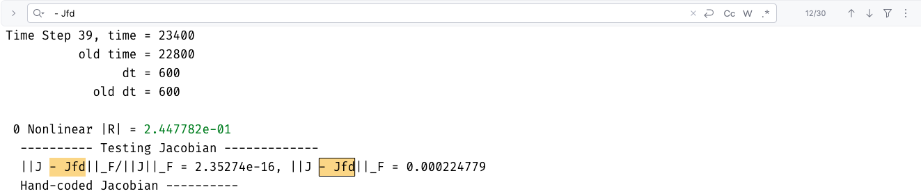
petsc_options = '-snes_test_jacobian -snes_test_jacobian_view'
Add this to executioner.
Forward file
- mesh
- variables
- usr_object, global param
Res 0
 It shows the correct grad for srv and perm 1e-20, 1e-12 But one iteration it jumps out. We need log scale.
2026-03-09
- not convergent, maybe due to the perm setup
- take a look at synthetic model. I suspect it’s not working well
- Why inversion is not passing the gradient to the main function, why I can not see the inner production between the adjoint wavefield an forward wavefield.
2026-03-11
I need you to help with my code. Currently I’m working on an inversion and I’m doing test on the synthetic model. I complete the forward modeling and adjoint by implementing @scripts/DSS_history_match/optimizer_input_file_test/perm3layer_fiberis/forward_and_adjoint.i and @scripts/DSS_history_match/optimizer_input_file_test/perm3layer_fiberis/optimize.i in MOOSE, and we can run this simulation with ease using conda env called “moose” in Python, then run this script we will get result in @scripts/DSS_history_match/optimizer_input_file_test/perm3layer_fiberis/optimize_out.csv which record the total misfit, and @scripts/DSS_history_match/optimizer_input_file_test/perm3layer_fiberis/optimize_out_OptimizationReporter_0001.csv which record the gradient to every parameter we want to optimize, I think these are the things you need to find an optimizer in Python and perform optimization, right? Then create a script in @scripts/DSS_history_match/optimizer_input_file_test/perm3layer_fiberis/optimization_prototype.py to run optimization for 10 times let’s see this method will work or not
2026-03-13
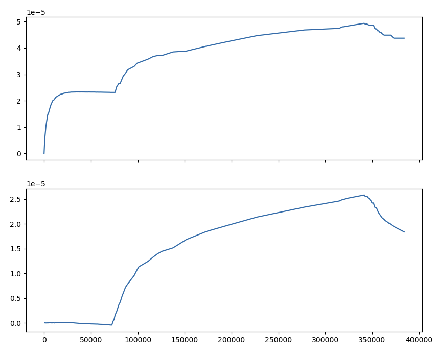
Working on validation.
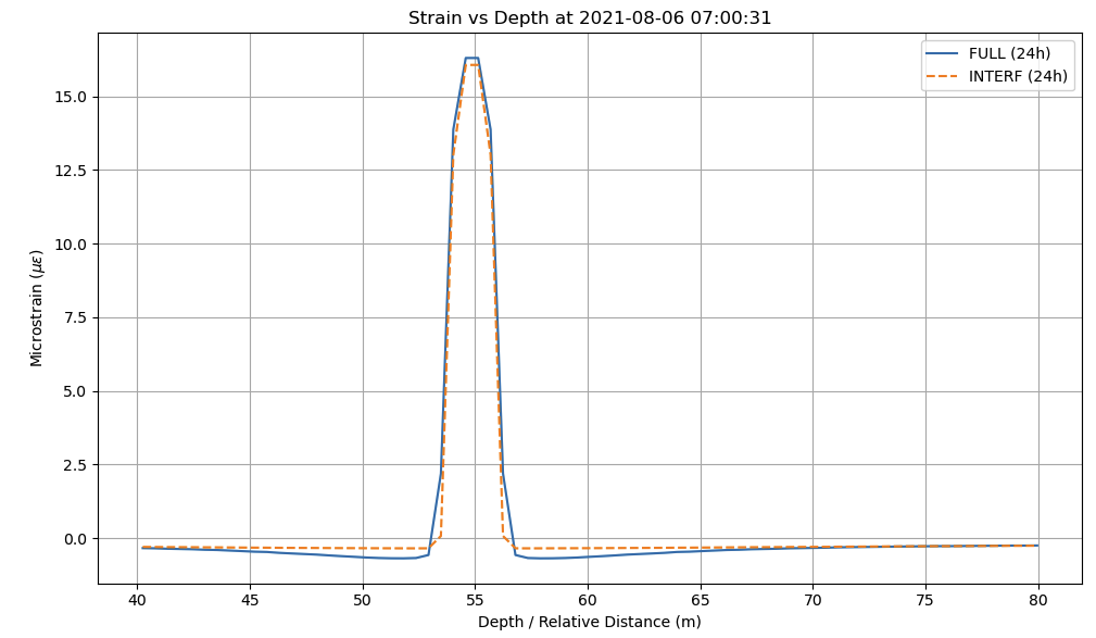
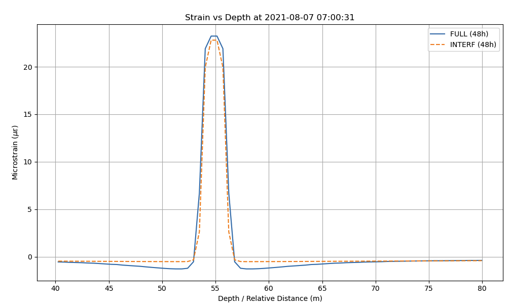
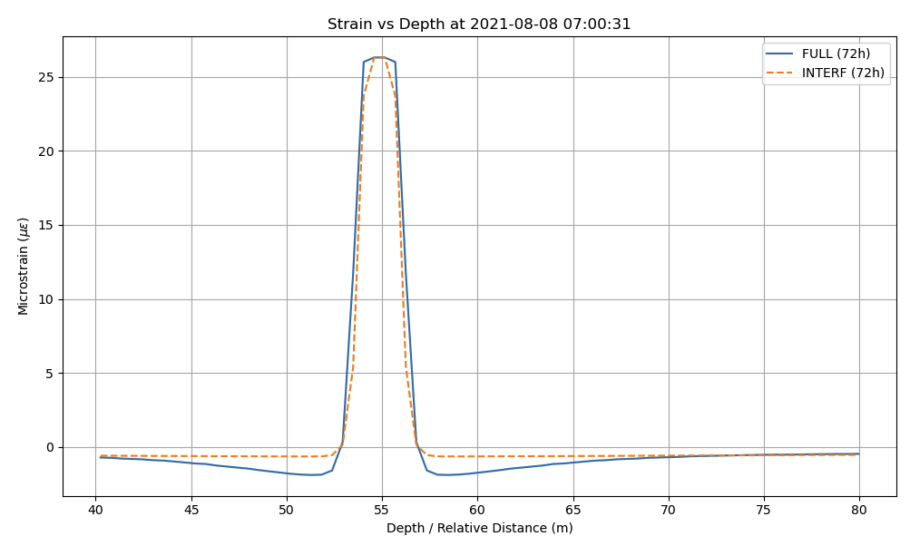
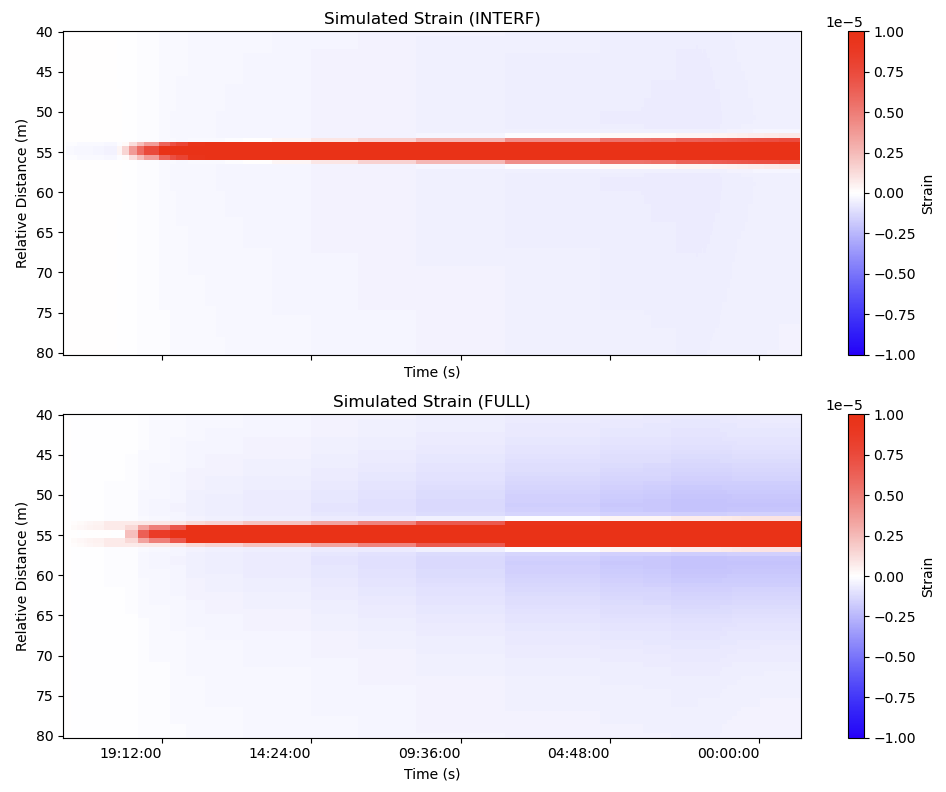
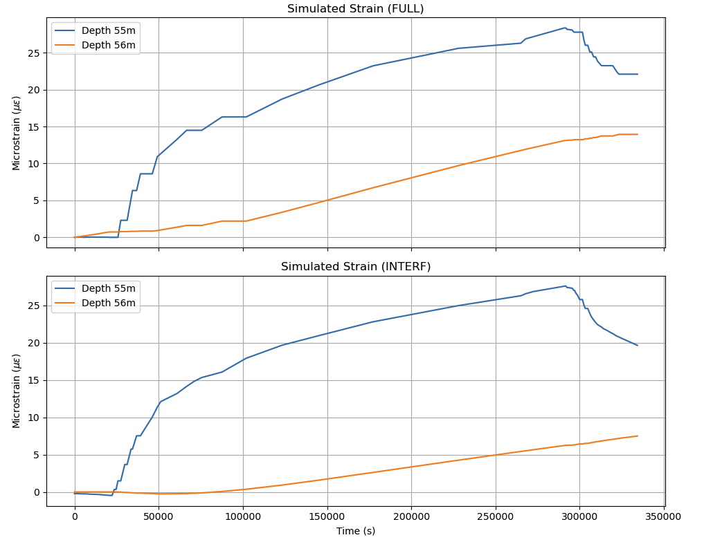
- full simulation vs only interference
- with mass_exp & without mass_exp
 End time:
 2021-08-09 03:51:59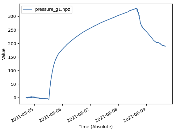
print(gauge_dataframe.get_end_time())
2021-08-09 16:07:42
2026-03-14 - prompt
Do you know 1. what is the interference test in oil and gas industry?
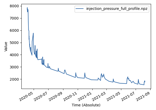
- how to simulate the strain change happened in fracture during interference test? If you know these questions, then here is what I’m confused in my project: currently, I’m trying to prove that in one way coupled diffusion system: $(\lambda + G)\nabla(\nabla \cdot \mathbf{u}) + G\nabla^2\mathbf{u} - \alpha \nabla p = \mathbf{0}$ and $\frac{\partial (\rho\phi_0)}{\partial t} - \nabla \cdot (\rho \frac{\mathbf{k}}{\mu} \nabla p) = 0$ we can skip the production period simulation but only to simulate interference to get the identical strain change signal (which is what we observed in fiber optic sensing). So to prove this I did numerical simulation on two different pressure profile, one is the figure starting from 2020(production + interference), another one is from 2021.8.6 (only interference). I use MOOSE to run the simulation, here is the python code for input files: xxx (file 1, 2) However, after I ran the simulation and then I extract the result and plot them, I found there are something wrong, the FULL simulation case shows a wrong signal (I say it wrong, because we did not observe such pattern in fiber optic sensing, but the only interference simulation one is correct). So my interpretation is the FULL simulation’s initial condition (I mean, the snapshot at the beginning of interference test) is wrong, because during the production period, you know because the matrix are of ultra low permeability (unconventional reservoir), so their pressure is dropping very very slightly, however, the fracture’s pressure is dropping just like what we observed in gauge data. So the pressure of fracture is confined by 1. the forced pressure boundary condition and 2. recharge of matrix. the second one will actually give a y direction displacement to the fiber which causes a always positive signal just like we observed (just my propose), so I am wondering how to solve this???
2026-03-16
2026-03-17
The mystery of optimizer
```yaml MOOSE Optimization: Single Forward+Adjoint Evaluation for External Optimizer
Problem
Need MOOSE to run exactly 1 forward + 1 adjoint solve (no internal
optimization iterations) so an external optimizer can consume the objective
and gradient.Key Findings
-tao_max_it does not work for this purpose:
- max_it=0 → PETSc crashes (“Maximum number of iterations must be positive”)
- max_it=1 → TAO runs 2 forward+adjoint pairs (iteration 0 = initial eval,
iteration 1 = one optimization step)
Solution: Set -tao_gatol to a very large value (e.g. 1e50)
TAO evaluates the gradient at iteration 0, sees gnorm < gatol, and declares
convergence before taking any optimization step. Result: exactly 1 forward + 1 adjoint.Executioner Configuration
[Executioner] type = Optimize tao_solver = taobqnls
petsc_options_iname = ‘-tao_gatol’ petsc_options_value = ‘1e50’
verbose = true
[]Verified Output (D = 0.01 0.01 0.01 0.01)
TAO SOLVER: iteration=0 f=1.11995 gnorm=37.452 cnorm=0 xdiff=1
total number of function/gradient evaluations=1
Solution converged: ||g(X)|| <= gatol- Objective: f = 1.11995
- Gradient norm: gnorm = 37.452
- Iterations: 0 (no parameter update)
- Forward+Adjoint pairs: 1
Notes
- verbose = true on the Executioner is needed to see TAO iteration info (f,
gnorm, etc.) - The -TAO_GATOL “unused option” warning is cosmetic — MOOSE parses and
applies the value internally before PETSc sees it. - The objective/gradient values are available in the OptimizationReporter for transfer to an external optimizer.
``` So conclusion, add “verbose=True” parameter in optimizer.2026-04-02
pre-conditioner too bad? ```yaml =================================================================================== = BAD TERMINATION OF ONE OF YOUR APPLICATION PROCESSES = PID 784777 RUNNING AT lakota.mines.edu = EXIT CODE: 9 = CLEANING UP REMAINING PROCESSES = YOU CAN IGNORE THE BELOW CLEANUP MESSAGES =================================================================================== YOUR APPLICATION TERMINATED WITH THE EXIT STRING: Segmentation fault (signal 11) This typically refers to a problem with your application. Please see the FAQ page for debugging suggestions
MOOSE run failed! Penalizing this step.
================================================== Optimization Result Summary: ================================================== CONVERGENCE: NORM OF PROJECTED GRADIENT <= PGTOL Success: True Final Objective: 10000000000.0 Optimized alphas saved to: /rcp/rcp42/home/shenyaojin/Documents/bakken_mariner/scripts/DSS_history_match/optimizer_input_file_test/perm5layer_100layer/inv/optimized_alphas.txt
If I use numps preconditioner, I got this;
I manually change the conditioner. Then?
```yaml
  1. Weak preconditioner (most likely)

  The default preconditioner (ILU/Jacobi) is too weak for your problem. Switch
  to a direct solver:

  [Preconditioning]
    [smp]
      type = SMP
      full = true
    []
  []

  And in your Executioner, use MUMPS:

  petsc_options_iname = '-pc_type -pc_factor_mat_solver_package'
  petsc_options_value = 'lu mumps'
Segment Fault
● Summary: Root Cause of the Segfault

  The TransientAndAdjoint executioner creates two separate nonlinear systems:
  nl0 (forward) and adjoint. Each system has its own matrix, solver, and
  preconditioner.

  The original [Preconditioning] block was:

  [Preconditioning]
    [smp]
      type = SMP
      full = true    # no nl_sys specified
    []
  []

  Without nl_sys, MOOSE doesn't know which system this preconditioner belongs
  to. It tries to apply full SMP coupling to the wrong system or in an invalid
  way — the adjoint system has different variables (pp_adjoint, disp_x_adjoint,
  disp_y_adjoint) than the forward system (pp, disp_x, disp_y), so the coupling
  structure is incompatible. This causes a null pointer dereference → segfault.

  The fix is to define separate preconditioners per system:

  [Preconditioning]
    [nl0]
      type = SMP
      nl_sys = 'nl0'
      petsc_options_iname = '-pc_type -pc_factor_mat_solver_package'
      petsc_options_value = 'lu mumps'
    []
    [adjoint]
      type = SMP
      nl_sys = 'adjoint'
      petsc_options_iname = '-pc_type -pc_factor_mat_solver_package'
      petsc_options_value = 'lu mumps'
    []
  []

  This also fixes the earlier linear solver stagnation issue — the default
  preconditioner (without the block) was too weak for the coupled PorousFlow +
  mechanics system. MUMPS direct solver on both systems gives robust
  convergence.
I’m not sure whether the optimizer is doing things correctly. So we need to test on the adjoint method. Let’s then apply the verbose option on for that three-layered model to see whether it will return a good result.
2026-04-03
Relook at the 3layer model, after adding a verbose option:
--- Evaluating parameters: [-15. -15. -15.] ---

---->

--- Evaluating parameters: [-15.00014079 -11.99079638 -15.00014509] ---
I’m more considering the numerical stability of the algorithm. 5 layered model, then how many layers I should set….?
2026-04-04
Prompt:
I need you to help me with the modeling scripts. First take a look at the
forward modeling script, which is designed to output a fiber's response on y
axis, which you can see from @scripts/DSS_history_match/optimizer_input_file_te
st/perm5layer_100layer/fwd/101_ground_truth.py the output extractor and
visualizer is ok not to look at. It generated the data in
"scripts/DSS_history_match/optimizer_input_file_test/perm5layer_100layer/data"
by script "scripts/DSS_history_match/optimizer_input_file_test/perm5layer_100la
yer/fwd/102_observation_extractor.py", then I would like to use the script to
invert from a initial permeability set, to reproduce the observation(forward
modeling made from ground_truth script). Then I wrote the script
@scripts/DSS_history_match/optimizer_input_file_test/perm5layer_100layer/inv/10
1_fiberis_inversion_model_loader.py which is the script builder for inversion,
then use @scripts/DSS_history_match/optimizer_input_file_test/perm5layer_100lay
er/inv/102_optimization_runner.py to run the INL MOOSE simulator. During the
inversion, I need to run forward, however, those forward modeling is not stable
 enough, the solver will start to loop and reach max iteration (2000) while
doing forward time step. Can you help me increase the stability of solving?
It's OK to take more time doing inversion, just need the result.
2026-04-07
● Clean. The changes:
- Removed SCALE_FACTOR, BASELINE_OBJ, and INITIAL_OBJ — no more artificial
scaling - Raw objective (~2.7e7) and raw gradient (~0.1 per component) go directly to
L-BFGS-B - With raw gradient ~0.1, L-BFGS-B’s first step will move alpha by ~0.07
(e.g., -18 → -17.93), which changes permeability by ~17% — enough for the
objective to respond and the line search to succeed (The update for the optimizer)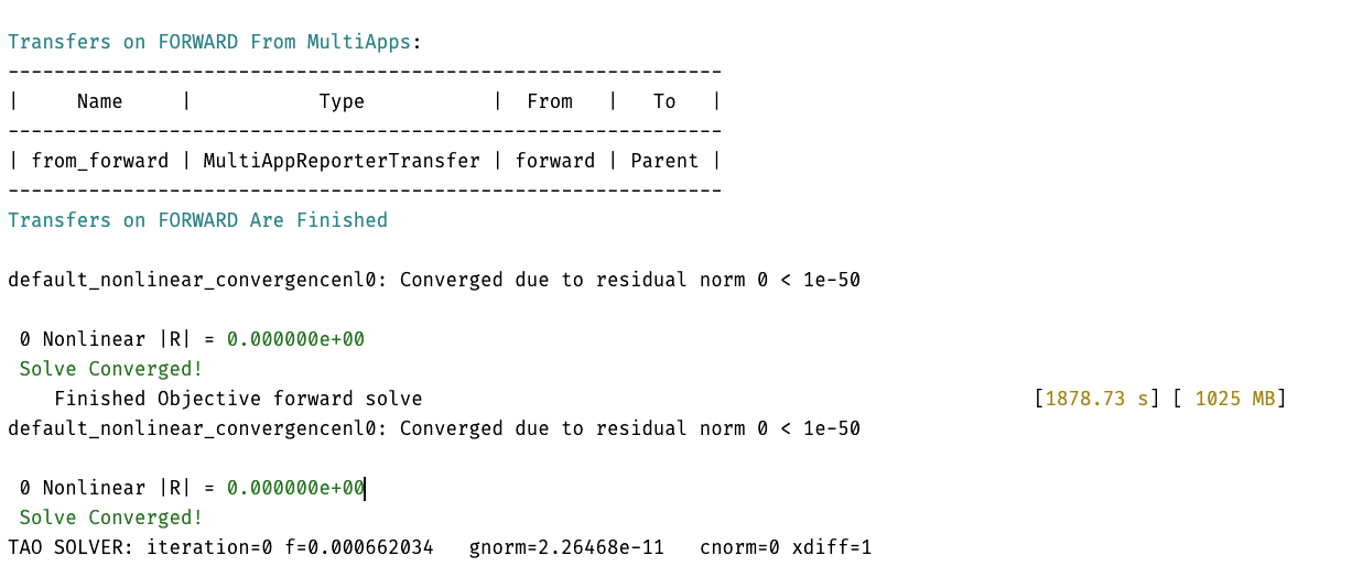 200 layer model; mesh size 200 * 200 = 1/2 hour 100 * 1/2 hour = ~2 days Summary from Claude
 We worked on the MOOSE optimization pipeline in fibeRIS/src/fiberis/moose/model_builder.py and scripts/DSS_history_match/.../inv/102_optimization_runner.py to get a permeability inversion working. Here's what was changed: 1. model_builder.py — Optimization Preconditioning Block Added add_preconditioning_block override in OptimizationLayeredModelBuilder that generates per-system preconditioners (nl0 + adjoint) with full = true and MUMPS LU, replacing the base class's single-system version. 2. model_builder.py — PiecewiseConstant → PiecewiseLinear Changed add_piecewise_function_from_data1d from PiecewiseConstant to PiecewiseLinear to eliminate step discontinuities in the injection pressure BC that were causing DIVERGED_LINE_SEARCH after 1 Newton iteration. 3. model_builder.py — Optimization Master File Executioner Changed the generate_optimization_master_file executioner to use tao_gatol = 1e50 so MOOSE TAO runs exactly one forward + one adjoint pass per call, letting scipy control the outer optimization loop. 4. model_builder.py — Attempted solve_type = NEWTON Added then removed solve_type = NEWTON because TransientAndAdjoint marks it as a private parameter. The full = true on SMP was sufficient to fix the convergence. 5. 102_optimization_runner.py — Scaling Iterations Multiple rounds of fixing the scipy L-BFGS-B optimizer scaling: - Removed SCALE_FACTOR = 1e9 — was inflating objective to ~1e16, causing all parameters to slam to bounds - Tried INITIAL_OBJ normalization — made gradient ~1e-19, steps too small. Removed. - Tried gradient-only chain rule compensation — mathematically inconsistent (objective and gradient don't match), breaks line search. Removed. - Final fix: OBJ_SCALE = 1e12 — scales both objective and gradient by the same constant. Consistent with minimizing C * f(x). Needed because 10^alpha parameterization at alpha=-18 produces gradients ~1e-12 (due to chain rule factor ln(10) * 10^(-18)). 6. 102_optimization_runner.py — Tolerances Set ftol = 1e-20, gtol = 1e-20, maxls = 10 to prevent premature convergence. 7. Diagnosed Bad Measurement Data Identified that 102_observation_extractor.py was writing the VPP id column (0, 0.1, 0.2...) instead of actual disp_y values (~1e-7 m) into the measurement CSV. User fixed this externally. Current Status The optimizer should now produce meaningful parameter updates. Next step: run 2-3 iterations and verify the objective decreases and SRV zone parameters move toward the ground truth (alpha ≈ -15 and -14.5).I’m running the scaled optimizer again, to see whether the optimizer will return me a correct gradient, then I can start to apply this to the real DSS-RFS data
2026-04-08
 Add part illustrating fracture-SRV-matrix → layered model
2026-04-16
2026-04-17
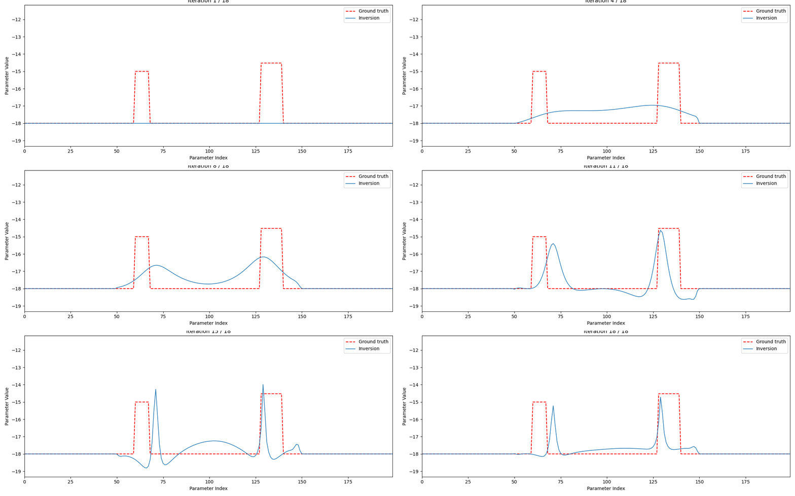
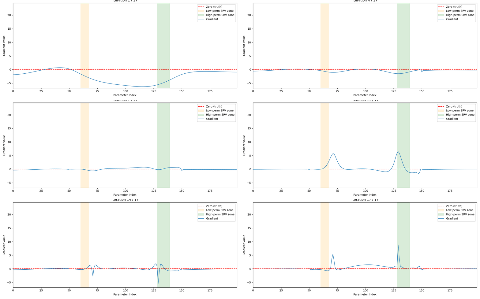
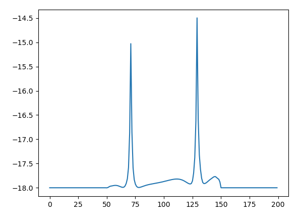
Running the inversion.
 Iteration 34,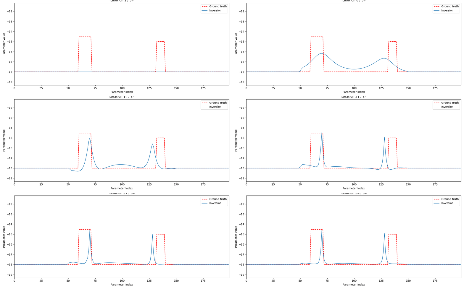
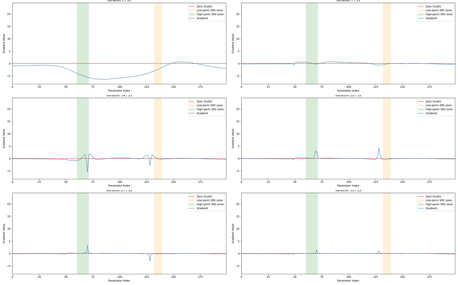 Done with the inversion. However, the inversion is not working while considering the
 disp_ybecause this physical measurement has inherit shortcoming.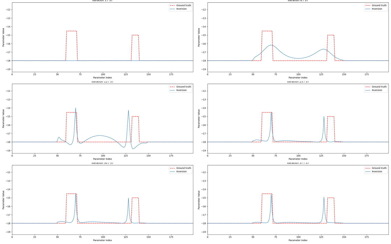
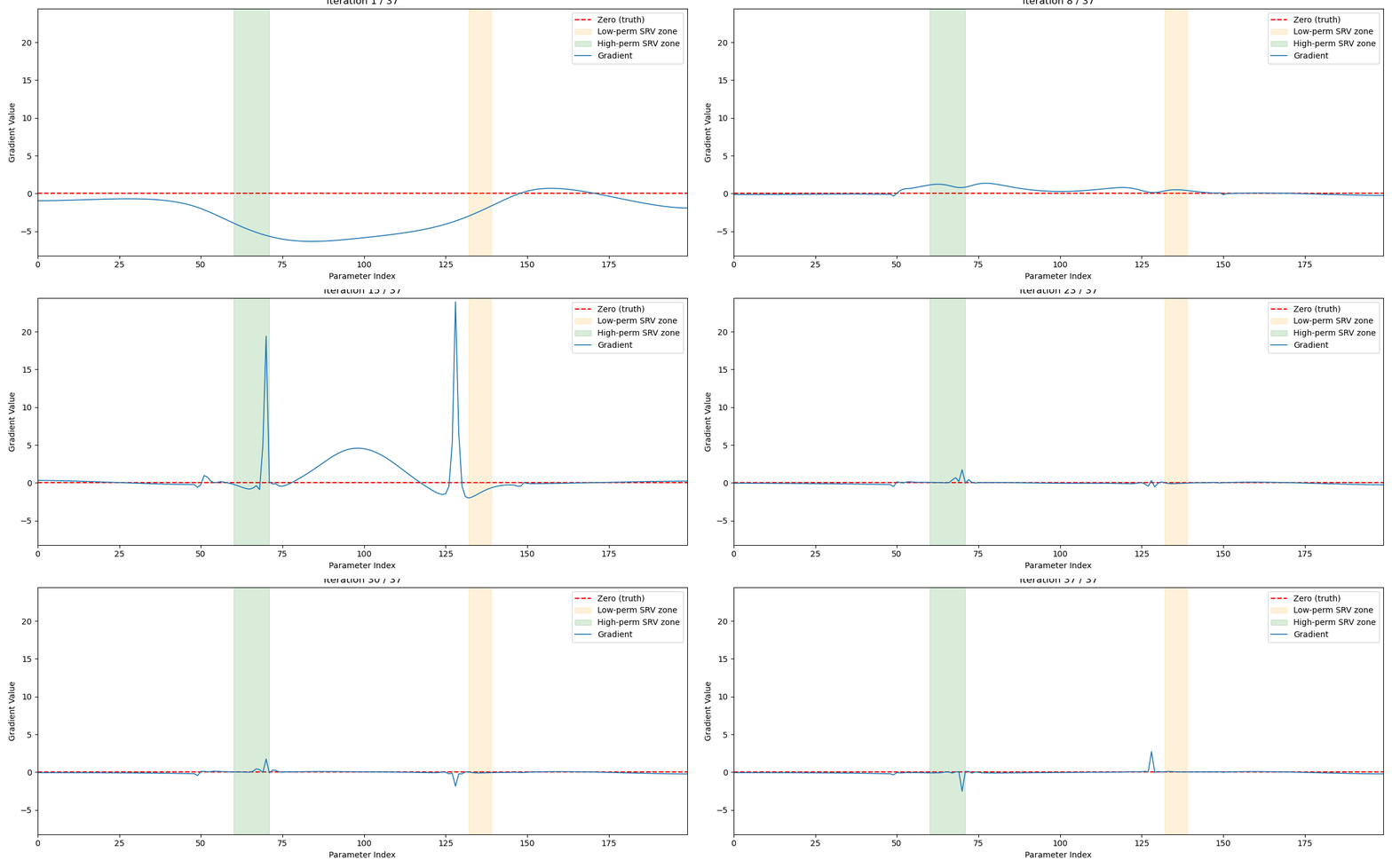 I’ll then start to write the algorithm to make the adjoint method to compare the strain directly. The Core Problem
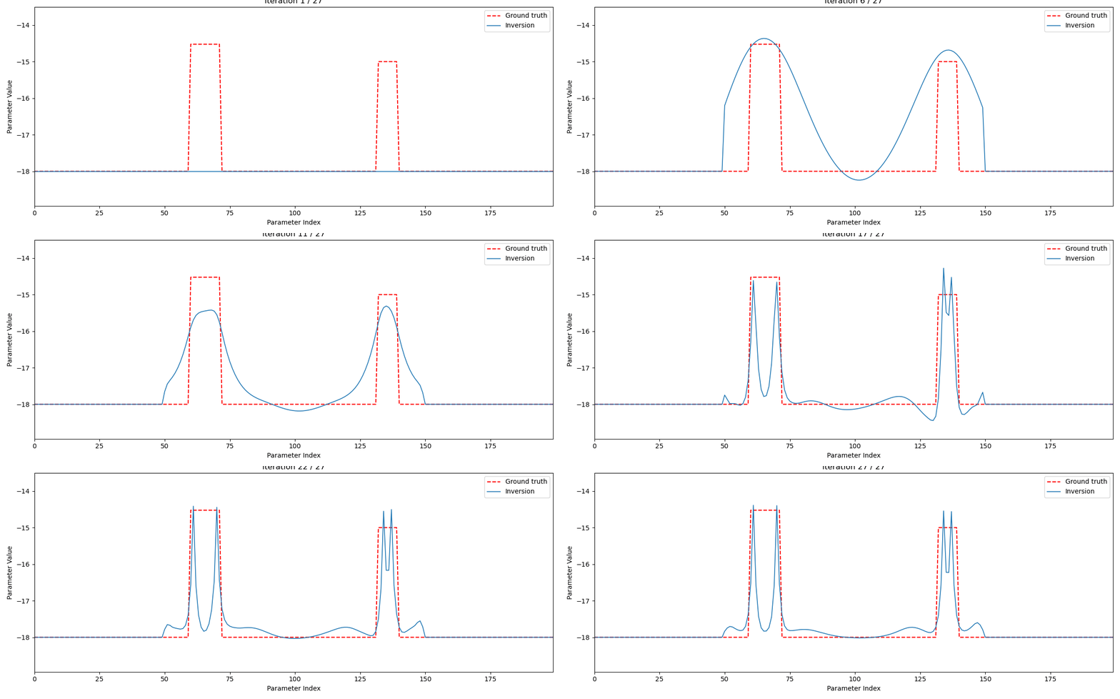
YourfibeRISinversion successfully recovered the correct permeability magnitudes ($\alpha \approx -14.5$ and $-15$) for the sandstone and shale layers, but it misplaced their depths. Instead of locating the true asymmetric anomalies at $y = -18$ and $+17$, the optimizer placed narrow spikes symmetrically at $y = \pm 14.5$.
The Investigation
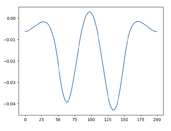
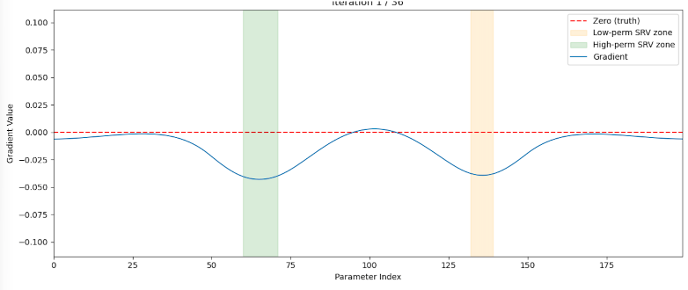
By analyzing theparameter_history.csvand comparing finite difference (FD) gradients to the adjoint gradients at the first iteration, it was discovered that the initial gradient didn’t point toward the true anomalies. Instead, it formed a single broad bowl centered in the domain ($y \approx +8$).
The Root Causes
The misplacement and altered shapes are the result of three compounding structural issues in the inversion setup:
1. Non-local Observation (disp_y): Displacement is the spatial integral of strain. A high-permeability band creates a “step” in the displacement profile, creating a large nullspace where shifting the anomaly’s depth slightly doesn’t significantly change the cumulative displacement above it.
2. Unfixed Rigid-Body Mode: With Neumann BCs on both ends, the vertical translation of the domain is unconstrained. This causes an unphysical gauge drift (DC offset) indisp_yover time, which the optimizer tries to fit, generating the artificial, center-peaked gradient bowl.
3. Regularization Artifacts: Trapped in this centered gradient bowl, the optimizer spreads outward until it hits the edges of the effective region ($\pm 14.5$). The prior and smoothness regularization then pinch these edges into narrow spikes rather than recovering the true, wider bands.
Why the Magnitudes Still Matched
The forward operator acts as a smoothing kernel (Green’s function). The amplitude of thedisp_ysignature is highly sensitive to the local permeability value but relatively insensitive to small spatial shifts. The inversion correctly matched the peak height of this smoothed signature to extract the right permeability values, but it traded off “where” and “how wide” the bands were within the kernel’s nullspace.
Recommended Action Plan
• Step 1 (The Quick Test): Add a single Dirichlet BC (e.g., pindisp_y = 0at a far corner like $y = -50$ or $+50$) to eliminate the rigid-body mode. This is a one-line change that will cleanly test if removing the gauge drift shifts the peaks toward their true locations.
• Step 2 (The Robust Fix): Switch the observation variable fromdisp_ytostrain_yy. Because strain is a local measurement, it natively resolves both the integration nullspace and the rigid-body drift. However, sincestrain_yyis anAuxVariable, this will require writing a customDiracKernel(roughly 100 lines of C++) to inject the adjoint source correctly, as MOOSE’sReporterTimePointSourceonly targets nonlinear variables directly.2026-04-21
2026-05-04
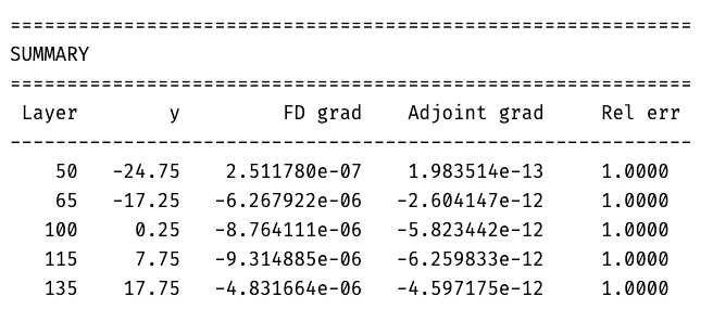
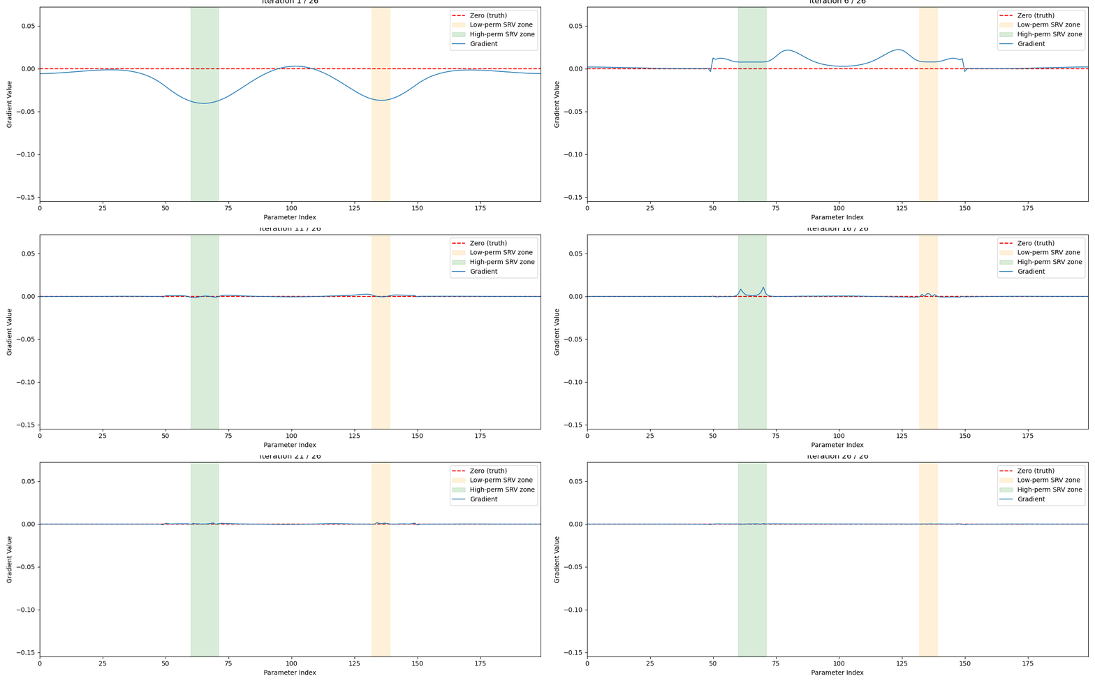
Wanna confirm the gradient is correct:
SUMMARY (eps = 0.1)
======================================================================
 Layer         FD grad    Adjoint grad        Adj/FD     Rel err
----------------------------------------------------------------------
    65   -3.755000e-08   -3.673302e-08    9.7824e-01     0.0218
   135   -4.135000e-08   -4.047876e-08    9.7893e-01     0.0211

Interpretation:
  At eps=0.5, Adj/FD was ~0.82 for these layers.
  If Adj/FD now -> 1.0, the previous gap was FD truncation (gradient exact).
  If Adj/FD stays ~0.82, there is a residual bias (likely the strain dipole h=0.5).
The running: ```python ● Bash(pgrep -af ‘mpiexec|combined-opt|102_optim|104_grad’ | head; echo “—”; ls /rcp/rcp42/home/shenyaojin/Documents/bakken_mariner/scripts/DSS_history_match/opti…) ⎿ — /rcp/rcp42/home/shenyaojin/Documents/bakken_mariner/scripts/DSS_history_match/optimizer_input_file_test/perm5layer_100_v2st rain/inv/optimize_temp.i
● Clean. Launching now:
● Bash(PYTHONPATH=/rcp/rcp42/home/shenyaojin/Documents/bakken_mariner/fibeRIS/src nohup /rcp/rcp42/home/shenyaojin/miniforge/envs/moose/bin/python 102_optimization_run…) ⎿ started pid=464824 —stdout head: Working directory : /rcp/rcp42/home/shenyaojin/Documents/bakken_mariner/scripts/DSS_history_match/optimizer_input_file_test … +12 lines (ctrl+o to expand)
● Bash(pgrep -af ‘python.*102_optim|mpiexec|combined-opt’ | head -3; echo “—file timestamps:”; ls -la /rcp/rcp42/home/shenyaojin/Documents/bakken_mariner/scripts/D…) ⎿ —file timestamps: -rw-r–r– 1 shenyaojin rcp 155272 May 4 2026 /rcp/rcp42/home/shenyaojin/Documents/bakken_mariner/scripts/DSS_history_mat ch/optimizer_input_file_test/perm5layer_100_v2strain/inv/inversion.stdout … +2 lines (ctrl+o to expand)
● Bash(pgrep -af ‘optimize_temp|combined-opt|102_op’ | head -3; echo “—”; ps -ef | grep -E ‘102_optim|combined-opt’ | grep -v grep | head -3) ⎿ — shenyao+ 464824 1 26 21:54 ? 00:00:04 /rcp/rcp42/home/shenyaojin/miniforge/envs/moose/bin/python 102_optimiza tion_runner.py … +5 lines (ctrl+o to expand)
● Running cleanly:
- python PID 464824
- mpiexec -n 20 PID 465001, with 20 combined-opt workers
inversion.stdout is growing (155 KB after 6 s = MOOSE streaming). objective_history.csv exists with the header; the first row will land at the end of iter 1 (~31 min).
Monitoring commands
One-line dashboard (re-run any time, no harm):
echo “— proc”; ps -o pid,etime,%cpu,rss,cmd -p 464824 2>/dev/null;
echo “— objective_history.csv”; column -ts, /rcp/rcp42/home/shenyaojin/Documents/bakken_mariner/scripts/DSS_history_match/optimiz er_input_file_test/perm5layer_100_v2strain/inv/objective_history.csv | head -20;
echo “— last MOOSE timestep:”; grep -E ‘Time Step|iteration=0’ /rcp/rcp42/home/shenyaojin/Documents/bakken_mariner/scripts/DSS_hi story_match/optimizer_input_file_test/perm5layer_100_v2strain/inv/inv_output/simulation_opt.log 2>/dev/null | tail -3
Live tail of the script’s stdout:
tail -f /rcp/rcp42/home/shenyaojin/Documents/bakken_mariner/scripts/DSS_history_match/optimizer_input_file_test/perm5layer_100_v2st rain/inv/inversion.stdout
Peek at current α (without disturbing the run):
/rcp/rcp42/home/shenyaojin/miniforge/envs/moose/bin/python -c “import numpy as np; a=np.load(‘/rcp/rcp42/home/shenyaojin/Documents/ bakken_mariner/scripts/DSS_history_match/optimizer_input_file_test/perm5layer_100_v2strain/inv/checkpoint_alpha.npy’);
print(‘mean=’,a.mean(),’min=’,a.min(),’max=’,a.max(),’\nactive layers (50-149) range:’,a[50:150].min(),’to’,a[50:150].max())”
To stop the run (if needed):
kill 464824 # graceful: python will tear down mpiexec children # if it doesn’t exit in 10s:
kill -9 464824 465001
What “healthy” looks like
After iter 1 completes (~31 min), objective_history.csv should show obj_raw ≈ 3.26e-6 (matching our FD-check baseline). After iters 2–5, obj_raw should be monotonically decreasing. If iter 2’s obj_raw ≥ iter 1’s, the line search is having trouble — first thing to check would be lowering BETA_* to 1e-10.
I won’t schedule a wakeup for this since it’s a multi-day run — just check on it whenever convenient.
We want to check the truncation error, then check the error in math, using the base definition of adjoint operator.
## 2026-05-06
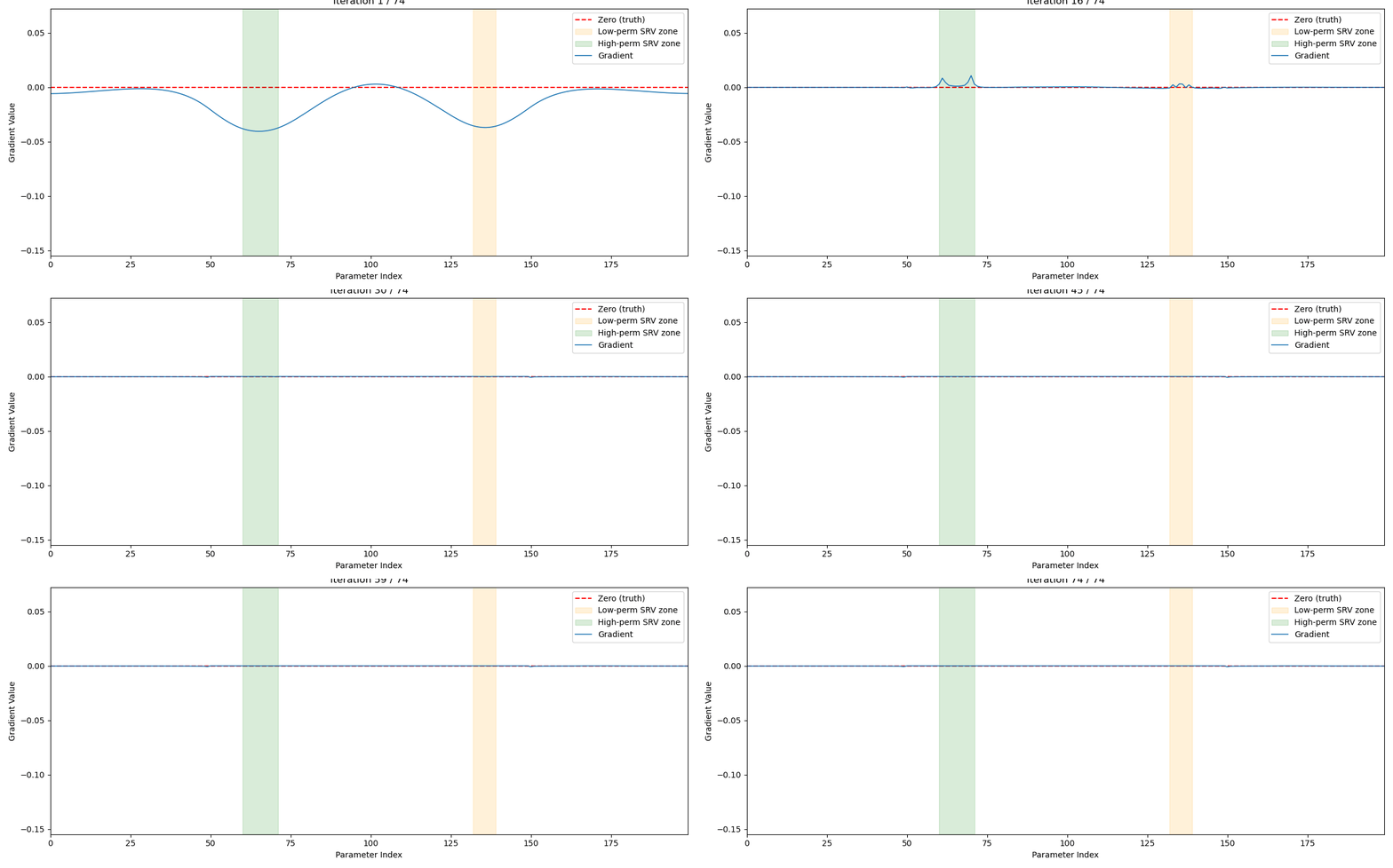
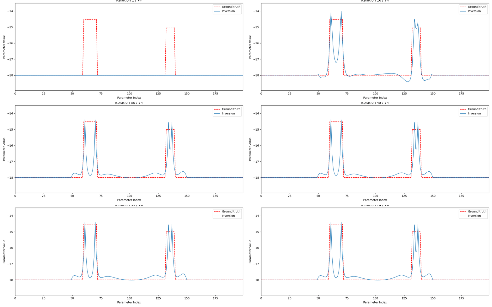
The optimizer finished running.
## 2026-05-28
I was trying on the TV reg. The initial result not seems good TBH. I will check the script done by claude to see where is the error.
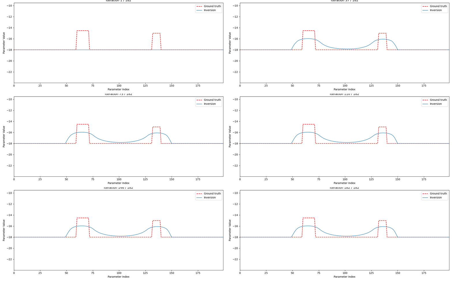
```shell
TV_RUN_MODE=truth_probe python scripts/DSS_history_match/optimizer_input_file_test/perm5layer_100_v2strain/inv/103_optimization_runner_TV.py
I ran that full MOOSE probe. Result: the raw data misfit at the true parameter is essentially zero:
obj_raw    = 1.1877249736e-33
reg_tv     = 2.2705794733e-06
obj_total  = 2.2705794733e-06
obj_scaled = 2.2705794733e+00
So the inversion workflow/data wiring is correct: when we insert the true parameter, MOOSE matches the synthetic observations. The nonzero total objective is entirely TV regularization, which confirms our earlier diagnosis that the TV term is what makes the optimizer prefer a smeared solution. 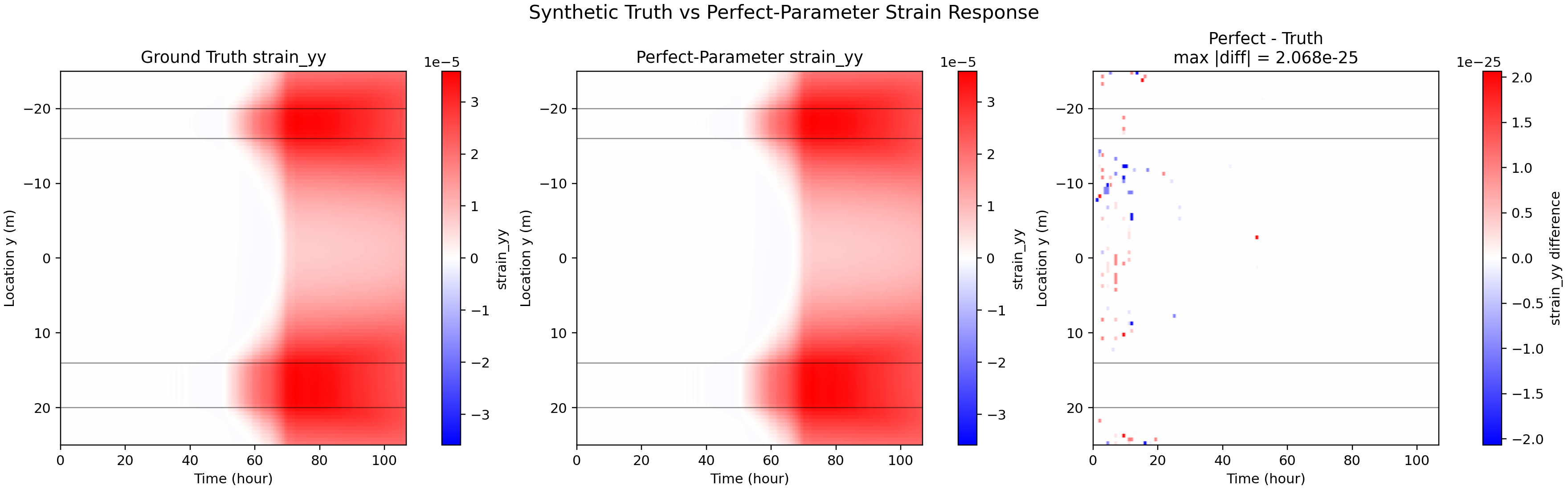
💡 Note
Looks like the workflow is totally right, but why TV reg is wrong? I also tried the tikhonov reg in scripts/DSS_history_match/optimizer_input_file_test/perm5layer_100_v2strain/inv/102_optimization_runner.py but it has spikes, can you help me qc the result by plotting the strain out. Then investigate the inversion workflow: why the reg is wrong?
2026-06-01
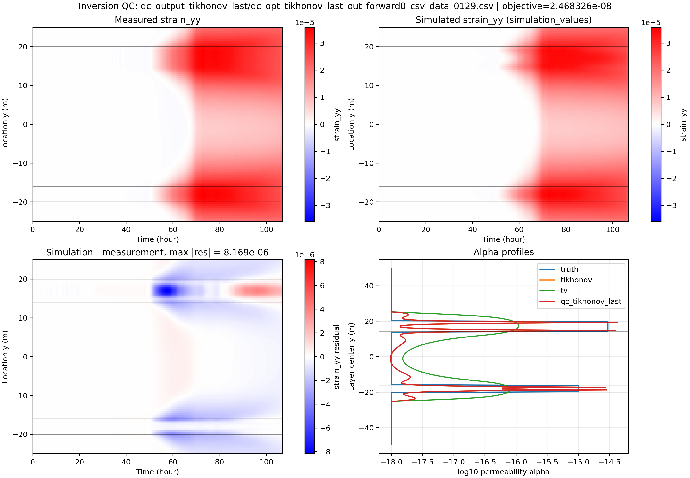
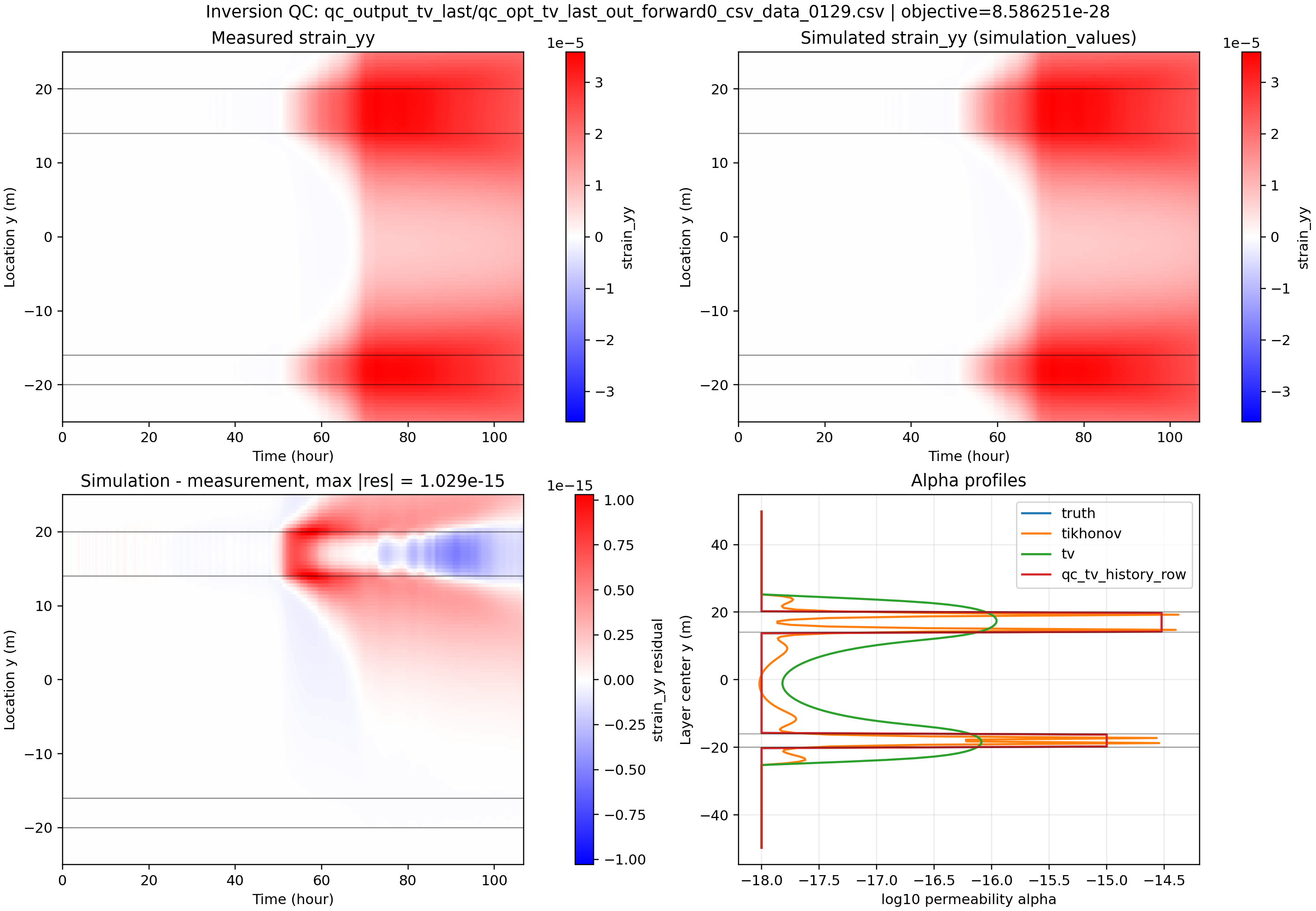 I compared TV reg and tikhonov reg, and here are the results. To understand how the gradients are calculated, please refer to: Regularization Tikhonov - perm inversion (internal note) TV reg - perm inversion (internal note) By the way, start model = all srv
PYTHONPATH=$PWD/fibeRIS/src ~/miniforge/envs/moose/bin/python scripts/DSS_history_match/optimizer_input_file_test/perm5layer_100_v2strain/inv/105_optimization_runner_no_reg_fracture_init.py
2026-06-03
I compare the intial model, using no reg term: 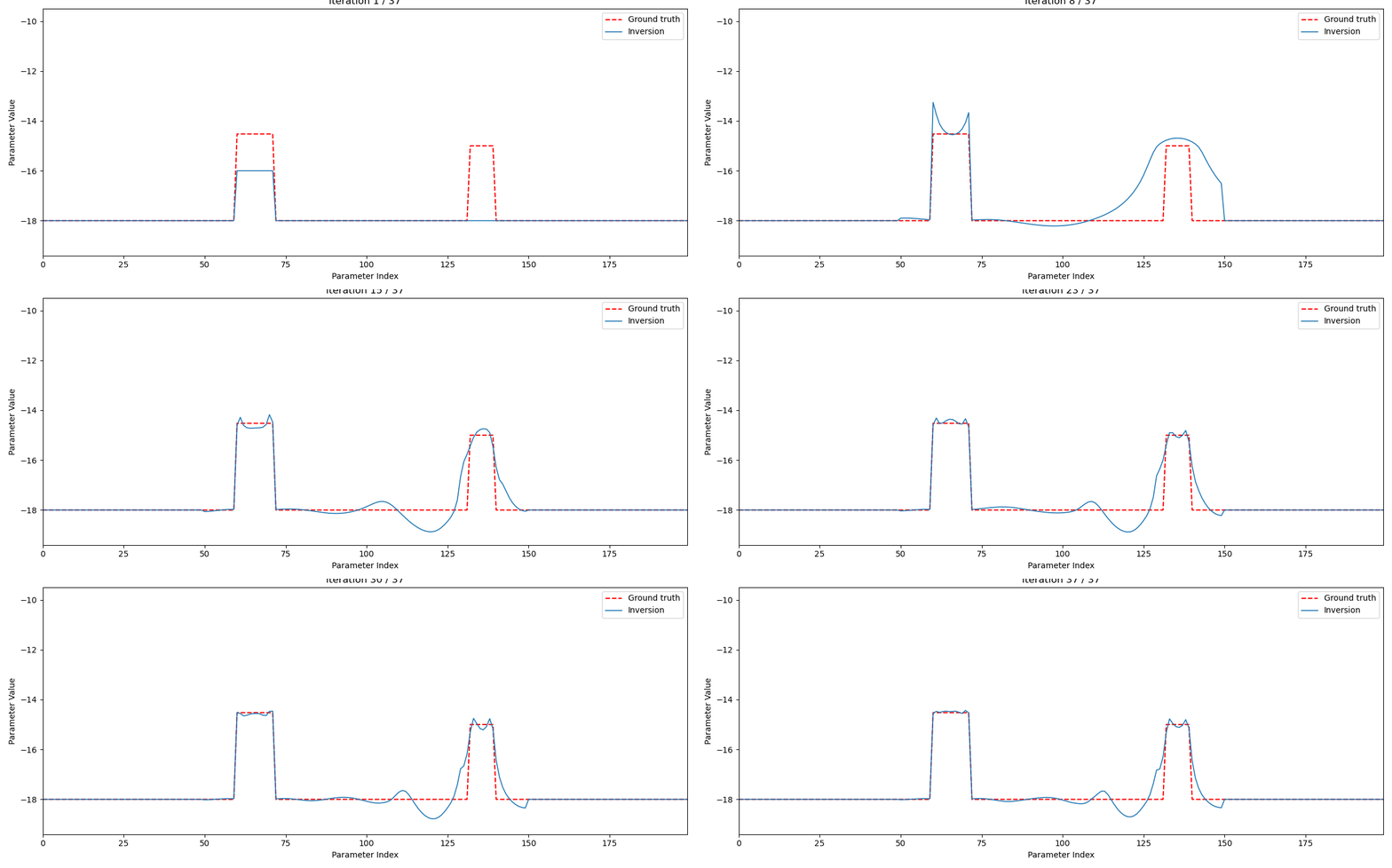 Left, I give a initial value to the SRV zone, even we don’t know the exact perm in that area, the inv will still return the correct shape&value of that, compared to the right one. I’m drafting the report to Jin. Report on permeability inversin 2026-06-03 (internal note)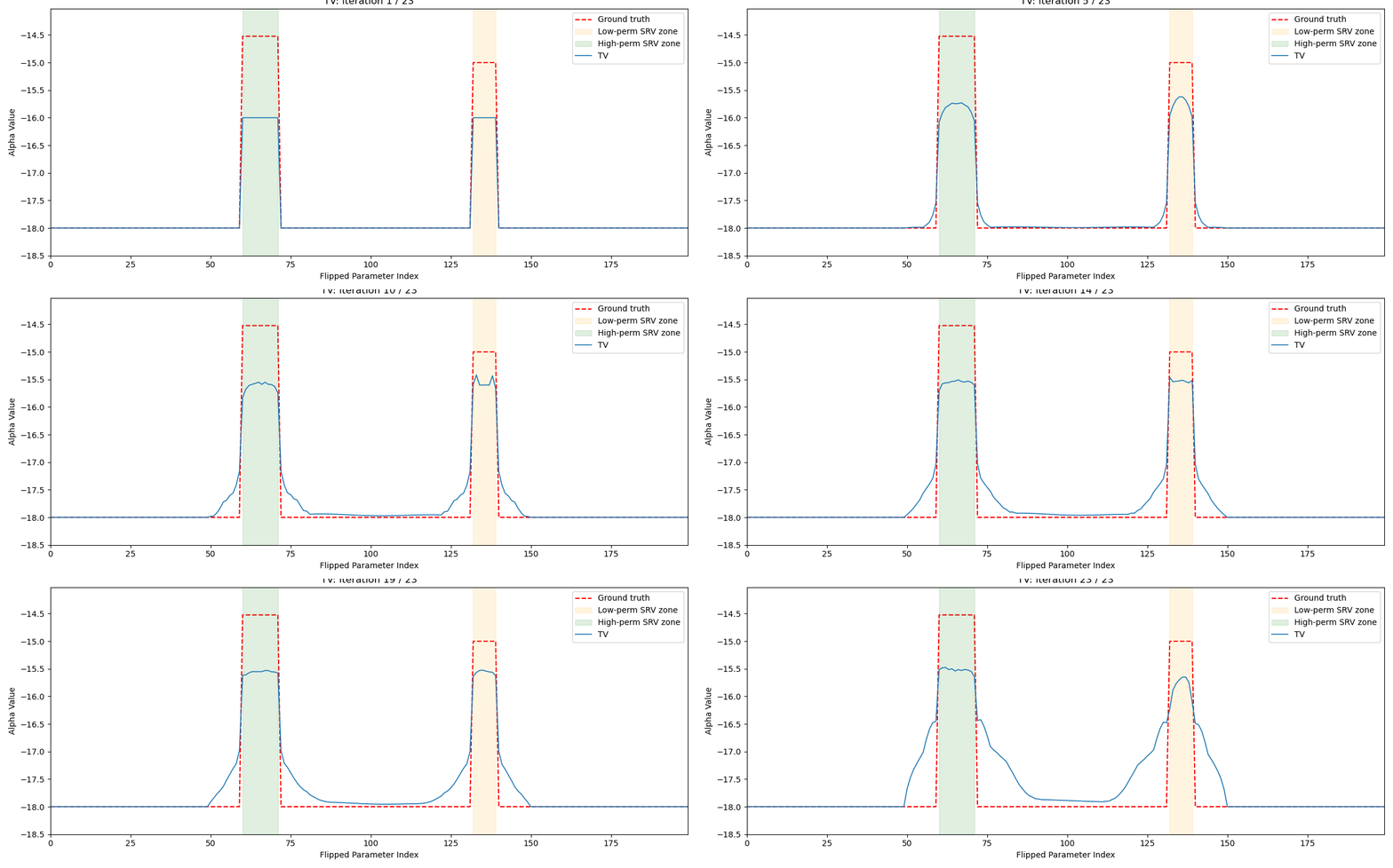
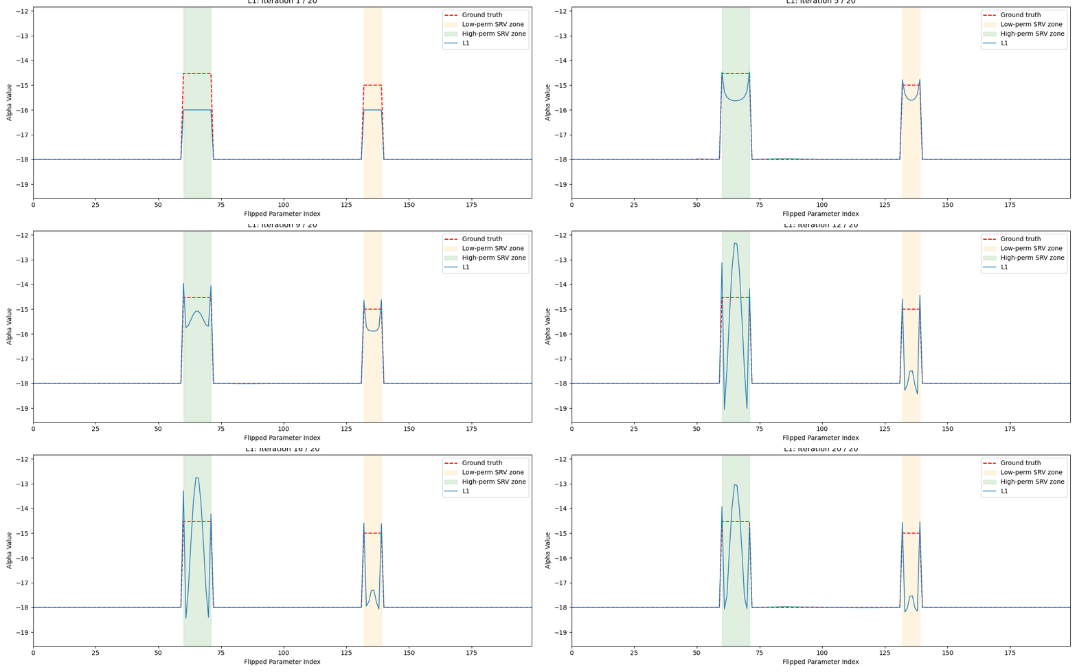 Under this coefficient:
BETA_TV  = 1e-7
DELTA_TV = 0.05
And,
BETA_L1  = 1e-9
DELTA_L1 = 0.05
I will shrink the coefficient L1 from 1e-9 to 2e-11. Originally, L1 is \(|\alpha_i - \alpha_{ref}|\) To use L-BFGS optimzier, we need tweak it, like this: \(\sqrt{(\alpha_i - \alpha_{ref})^2 + \Delta_{L1}^2} - \Delta_{L1}\)
2026-06-08
Obj scaled: 0.0013
||grad|| raw=1.3943e-11  scaled=1.3943e-05
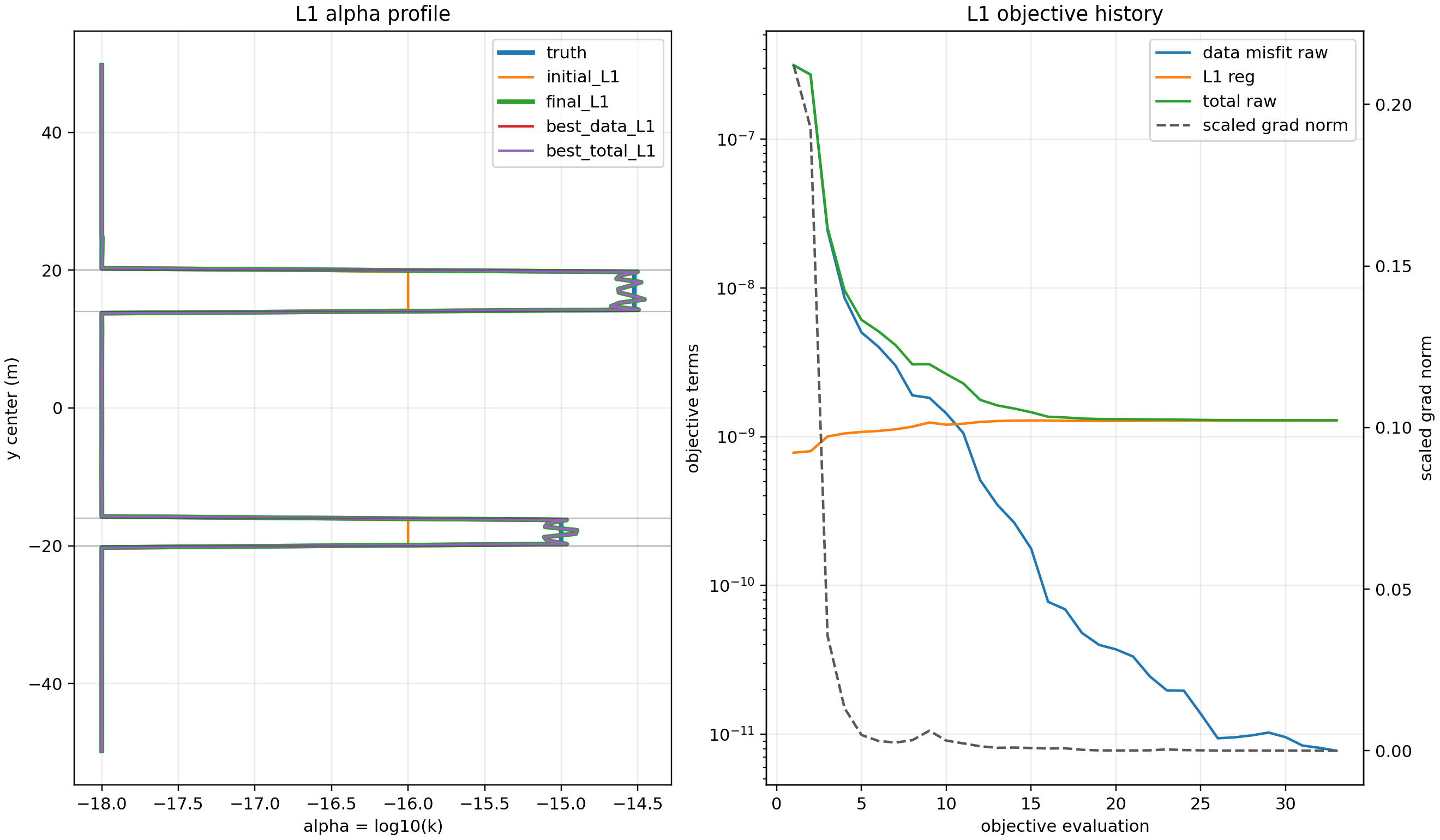
New best data-fit alpha saved to: /rcp/rcp42/home/shenyaojin/Documents/bakken_mariner/scripts/DSS_history_match/optimizer_input_file_test/perm5layer_100_v2strain/inv/best_data_alpha_L1.txt
New best total-objective alpha saved to: /rcp/rcp42/home/shenyaojin/Documents/bakken_mariner/scripts/DSS_history_match/optimizer_input_file_test/perm5layer_100_v2strain/inv/best_total_alpha_L1.txt
Accepted step 30: ||dx||=7.5627e-03, max|dx|=3.0861e-03, small_step_count=2/3

==================================================
Optimization Result Summary (L1):
==================================================
CONVERGENCE: RELATIVE REDUCTION OF F <= FACTR*EPSMCH
Success       : True
Stopped by step tolerance: False
Final Objective: 0.001289283110964436
Optimized alphas saved to: /rcp/rcp42/home/shenyaojin/Documents/bakken_mariner/scripts/DSS_history_match/optimizer_input_file_test/perm5layer_100_v2strain/inv/optimized_alphas_L1.txt
Here is the output from L-BFGS; below is the result from L-1 reg. 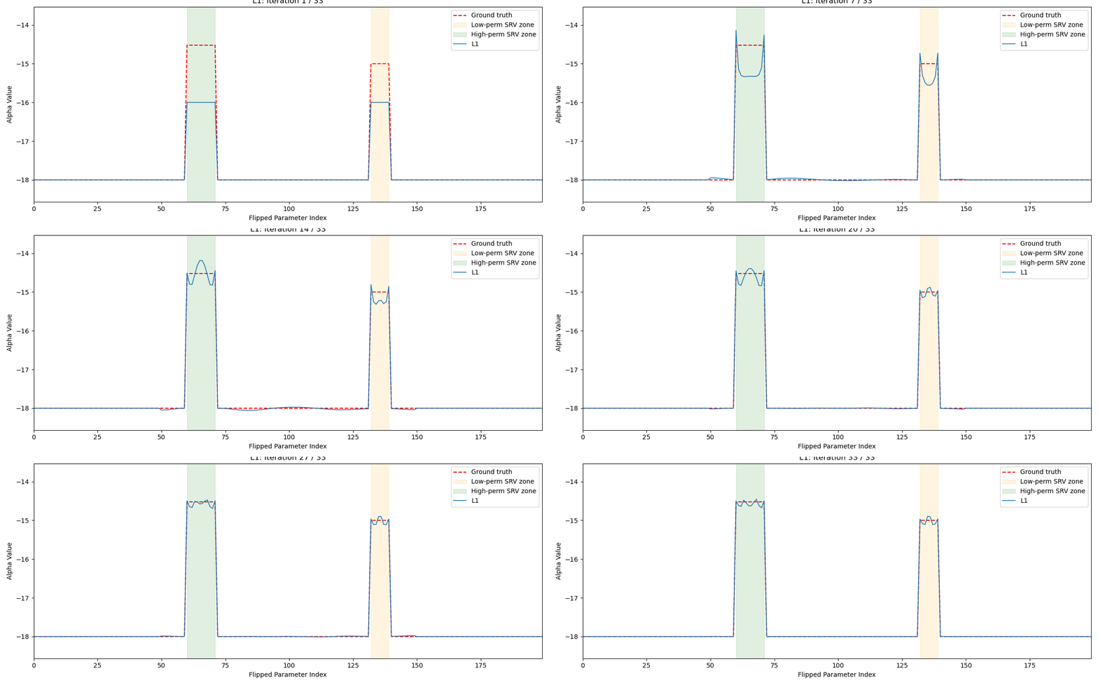 Here is the QC plot for the synthetic data.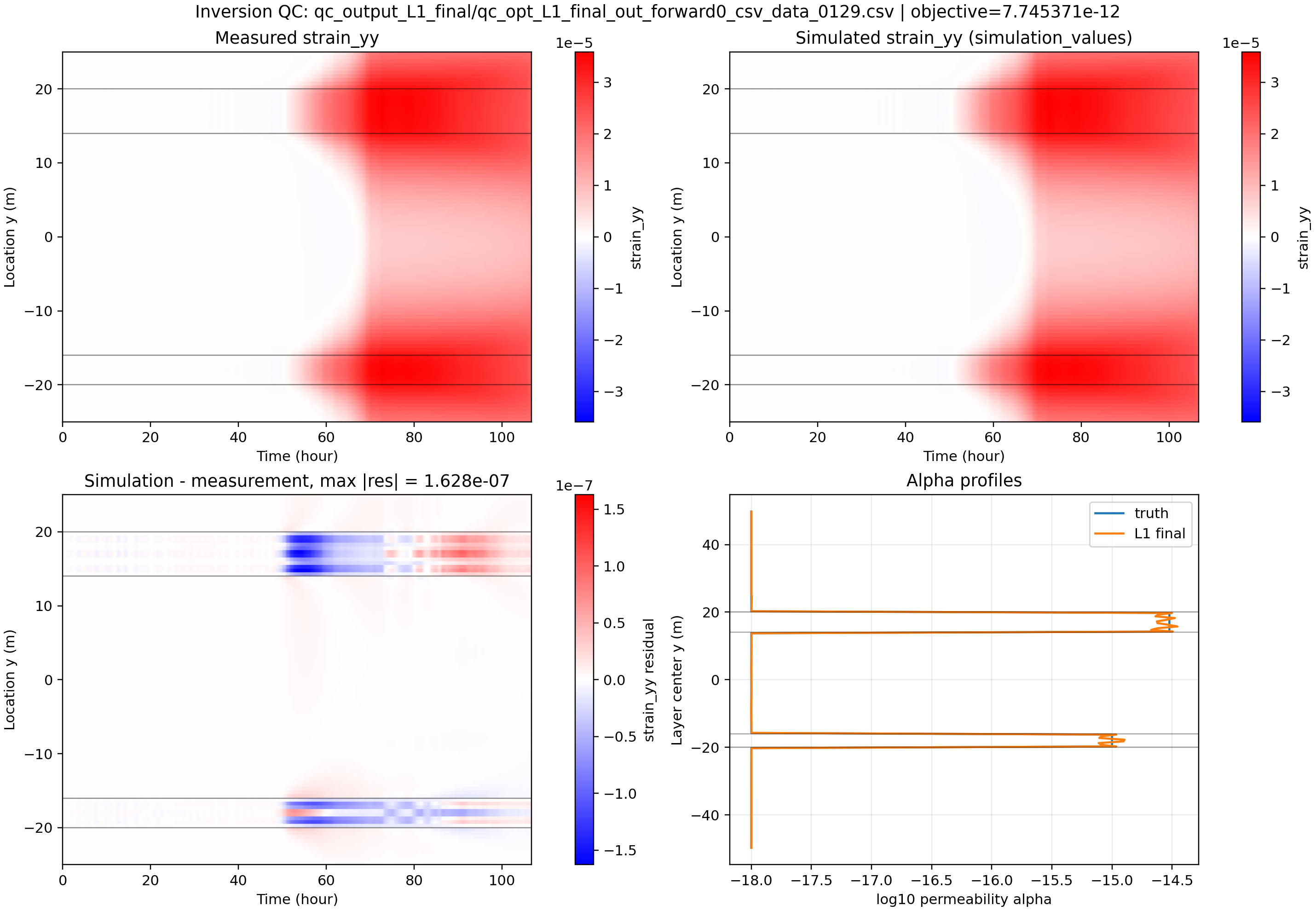
2026-06-12
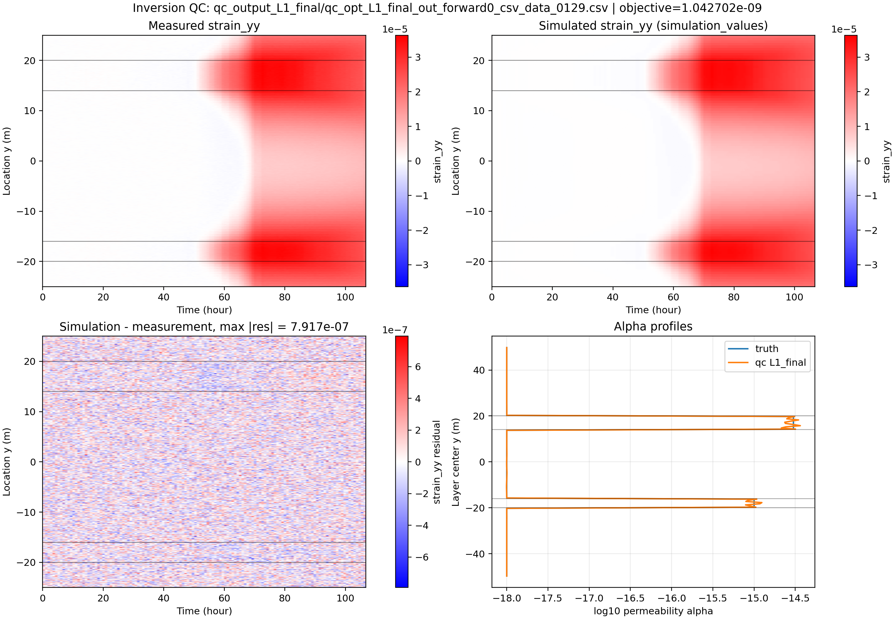
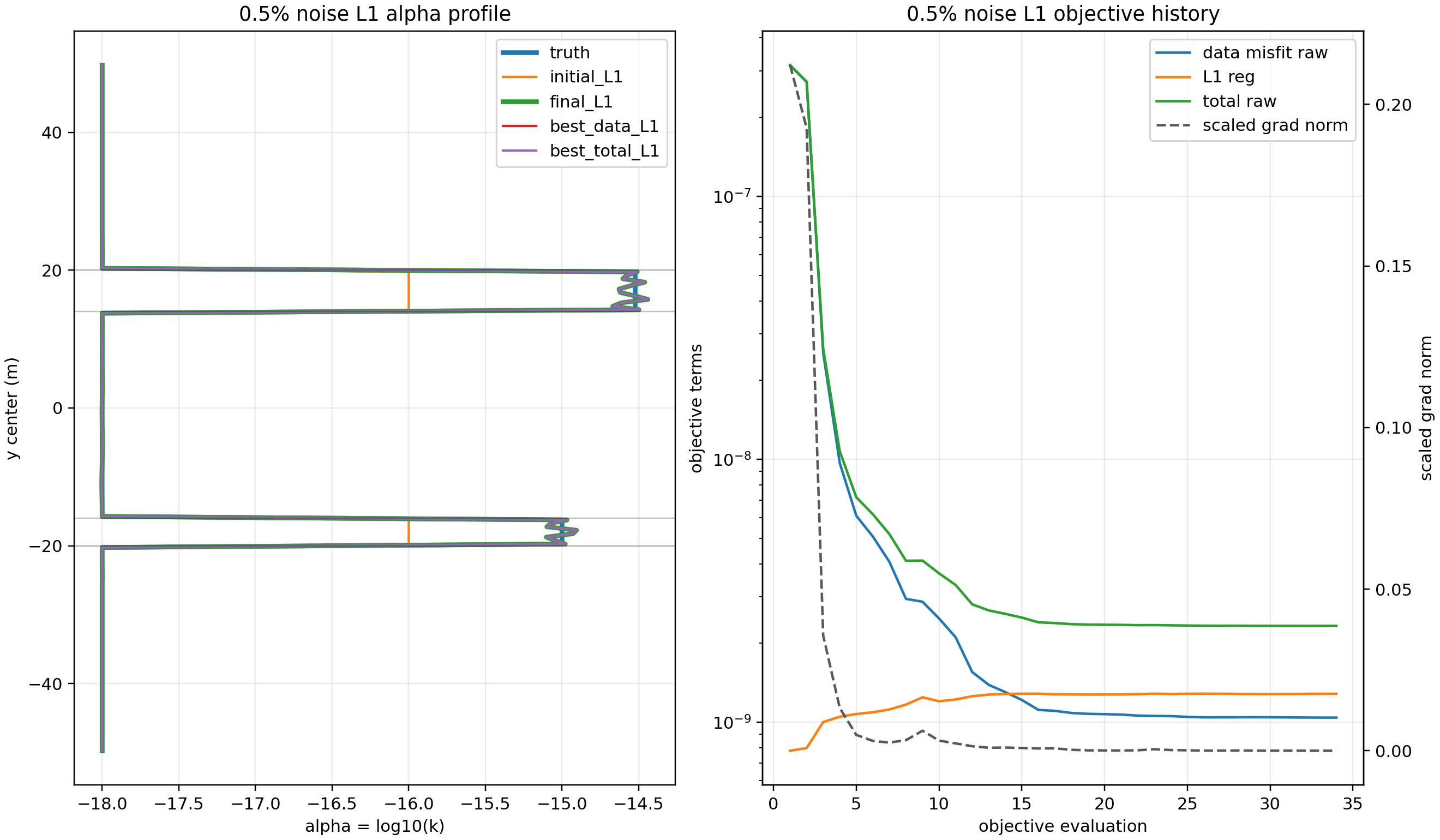
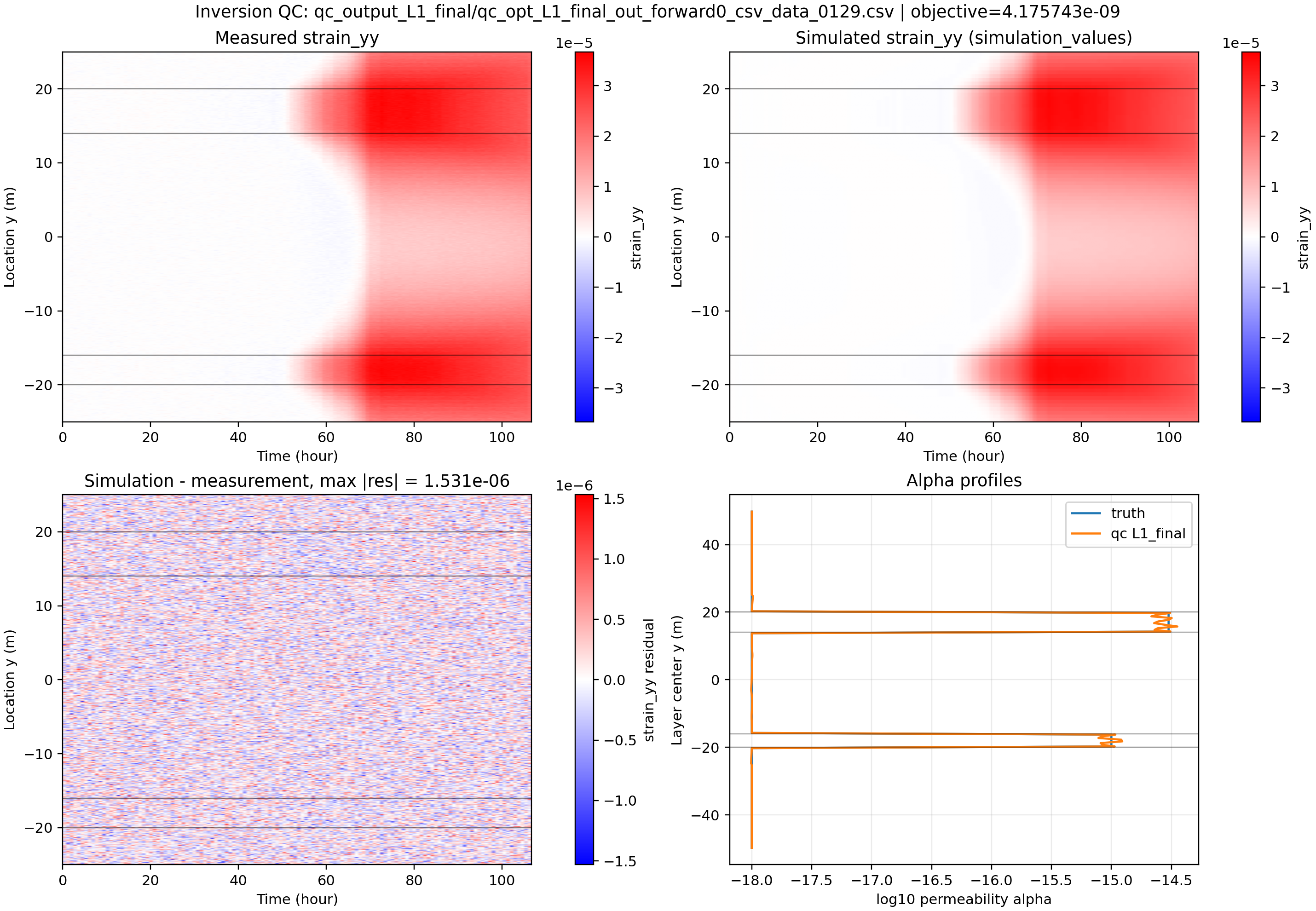
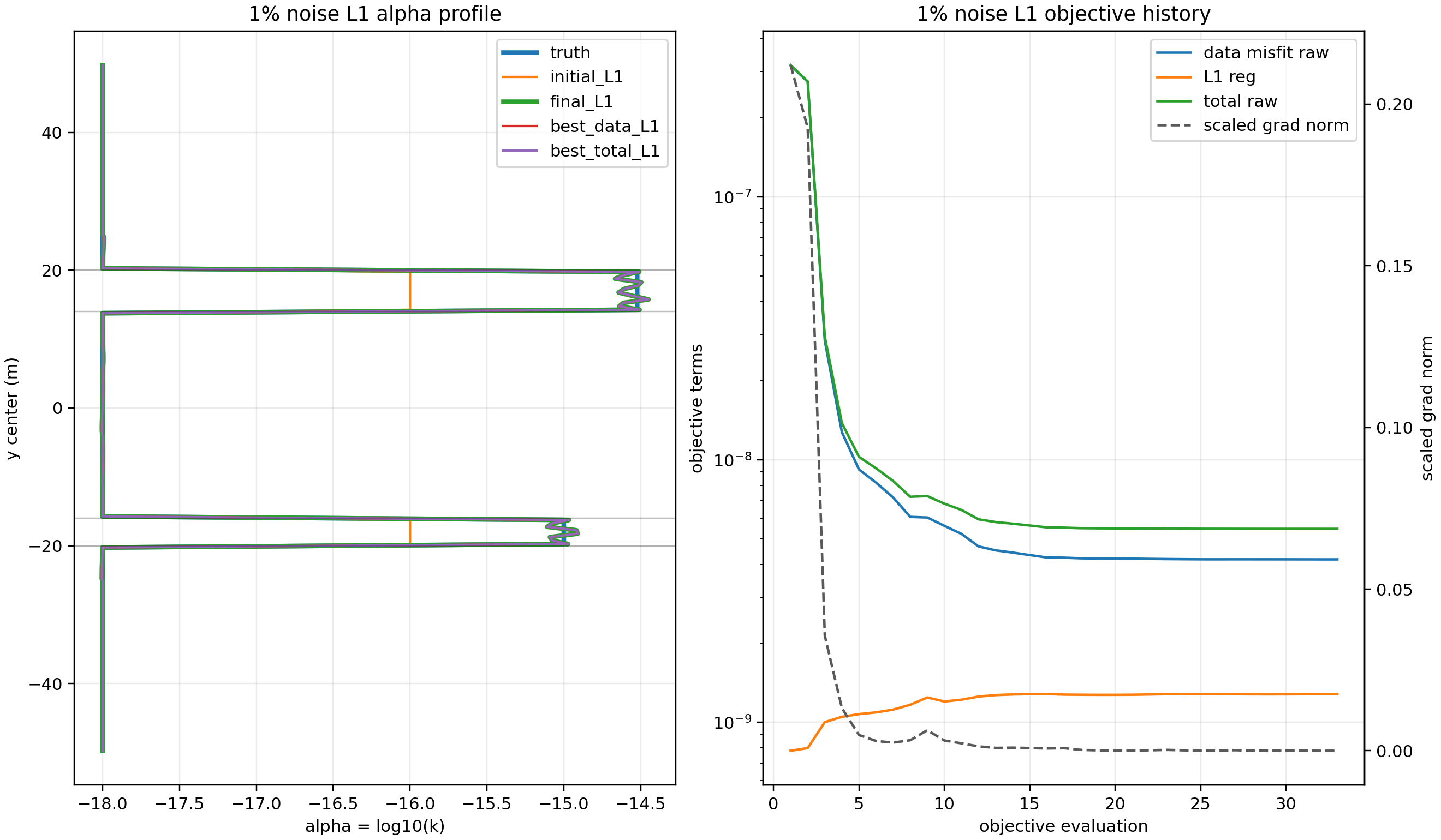
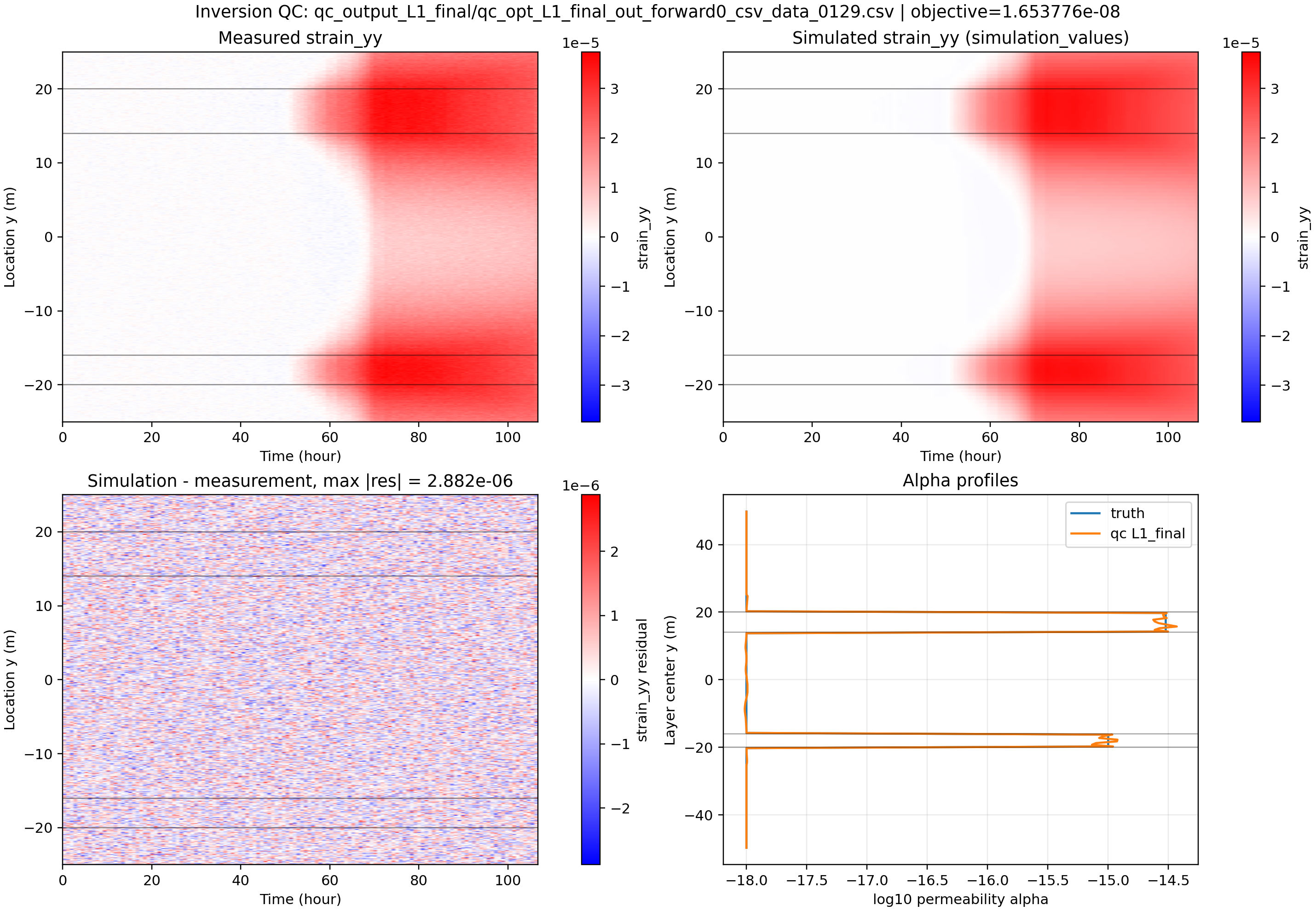
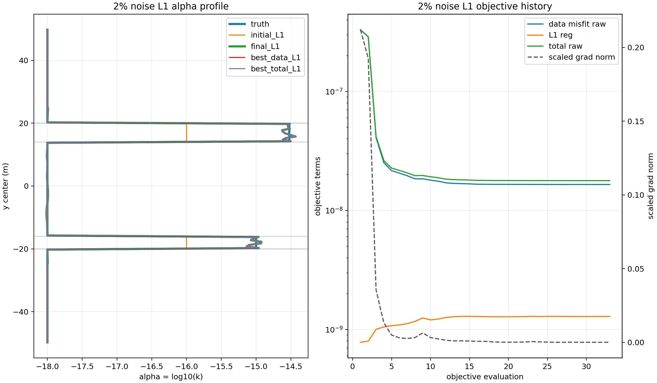
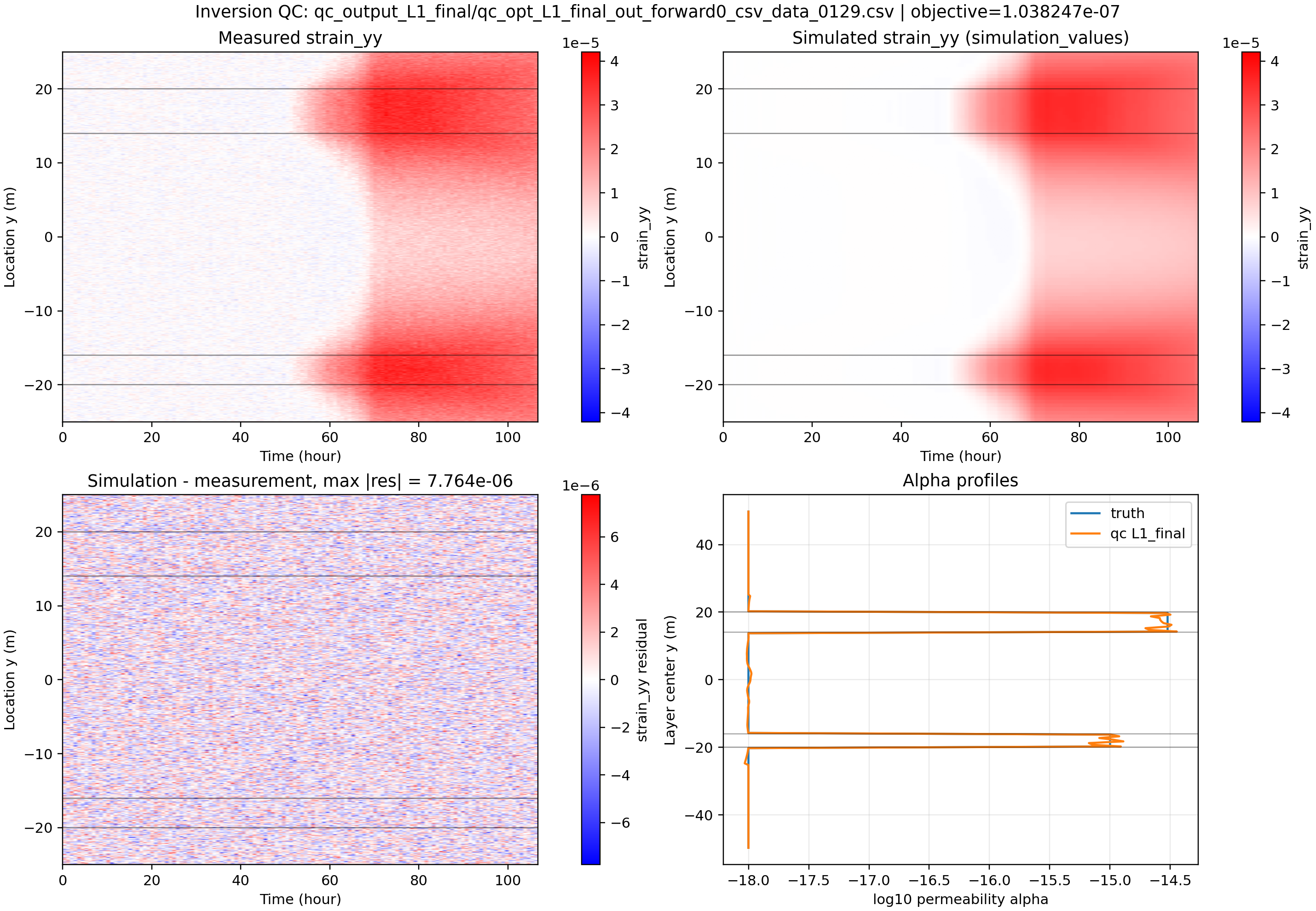
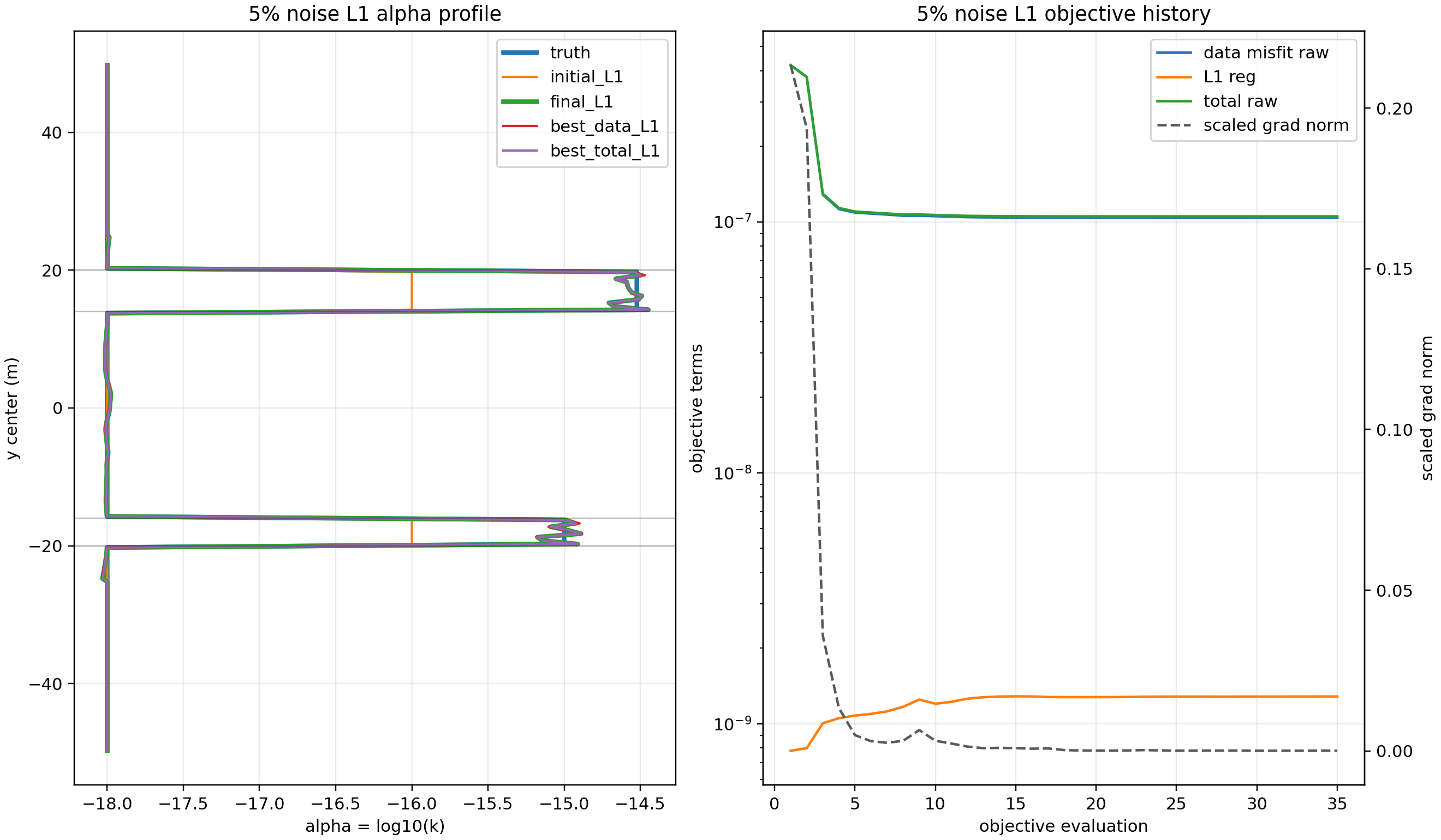
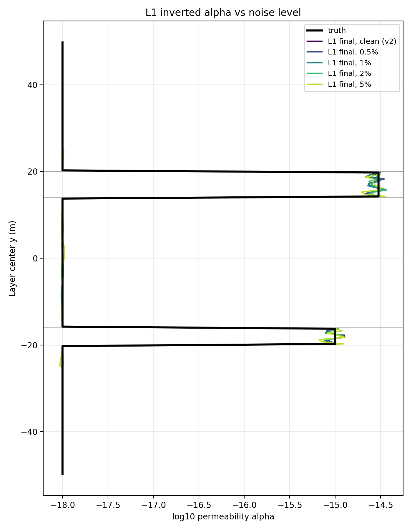
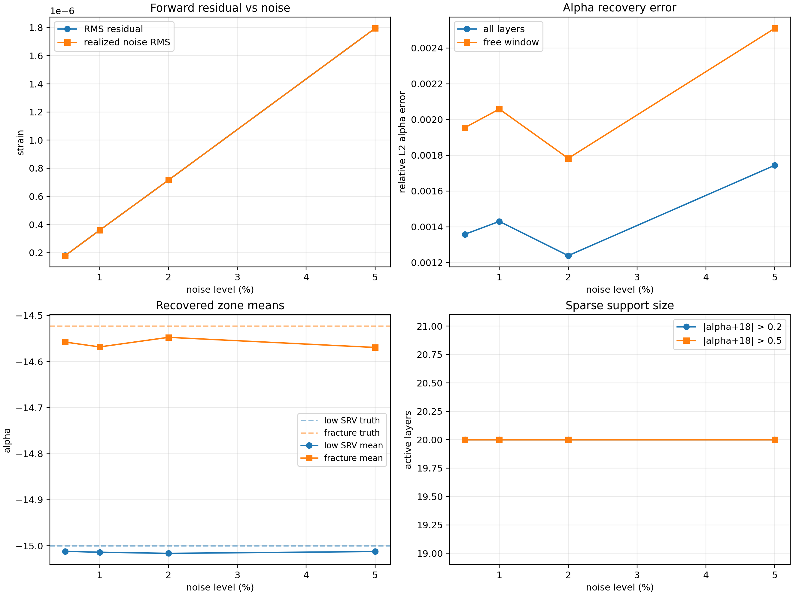
I add the noise in this way: Adds Gaussian noise to measurement_values with std = pct · max|d| (max|d| = 3.589e-5), applied to all points, independent per-level seeds. I have finished to test adding noise to the model.
noise level = 0.5 pct
noise level = 1 pct
Noise level = 2 pct
Noise level = 5 pct
Result = all
- todo: add median noise
- Todo: add poisson noises
Enjoy Reading This Article?
Here are some more articles you might like to read next:
- History Matching with DSS: Is Diffusion Linearly Additive?
- How to deploy a blog using the code in this repository?
- MOOSE PorousFlow: Governing Equations
- Dialogue Log: Debugging a MOOSE Script with Gemini
- fiberis.analyzer philosophy
- fiberis.moose setup
- Cement Shrinkage and Microannulus Formation in Horizontal Wells
- fiberis.moose: Programmatic MOOSE Input Generation
- Pressure Diffusion in Fractured Media
- Poisson's ratio test python code